7 Saving the resulting image

7.1 ggkeggsave

ggkegg uses the annotation_raster for overlaying the original KEGG image. This section describes how one can save the resulting custom plot for the publication. The ggkeggsave function is prepared, which respects the original dimension of the image. The function is intended for the ggplot with the overlay_raw_map layer. On overlay_raw_map, one can control whether the interpolation is performed by interpolate option. In some instances, interpolate=TRUE makes blurry images, and please try to disable the interpolation in that case.

library(ggkegg)
library(ggh4x)
g <- pathway("hsa04130")
gg <- ggraph(g, layout="manual", x=x, y=y)+
    geom_node_rect(aes(fill1=x, filter=type=="gene"))+
    geom_node_rect(aes(fill2=y, xmin=xmin+width/2, filter=type=="gene"))+
    scale_fill_multi(aesthetics = c("fill1", "fill2"),
        name = list("Condition1", "Condition2"),
        colours = list(
            scales::brewer_pal(palette = "RdBu")(6),
            scales::brewer_pal(palette = "RdPu")(6)),
            guide = guide_colorbar(barheight = unit(50, "pt")))+
    overlay_raw_map()+
    theme_void()
ggkeggsave("test1.png", gg)
knitr::include_graphics("test1.png")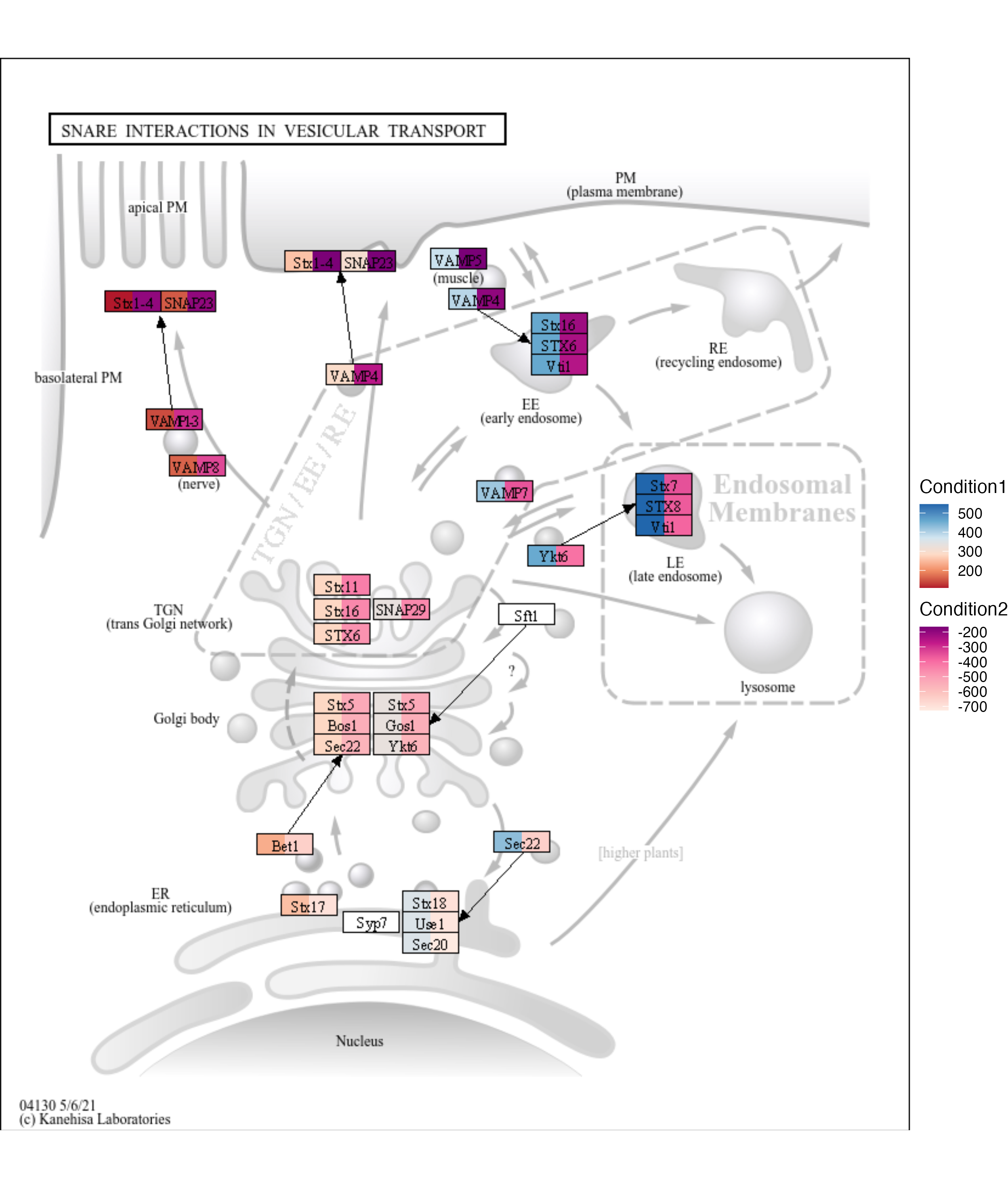

7.2 output_overlay_image

If one wants to keep the original resolution of the image, output_overlay_image function can be used. This combines the image from ggplot layers and the original PNG image (and optionally legend image) and outputs it. This extracts the main panel from ggplot objecy by gtable functions, and thus the legend, title, axis and the other elements outside the main panel is omitted for aligning the node position with the original image. The legend can be placed inside the plot by the theme like theme(legend.position=c(0.5, 0.5)), or with_legend_image=TRUE can be specified to additionaly concatenate the legend image.

The examples follow:

The legend insides the main panel.

g <- pathway("hsa04130")
gg <- ggraph(g, layout="manual", x=x, y=y)+
    geom_node_rect(aes(fill=x, filter=type=="gene"))+
    theme_void()+
    theme(legend.position=c(0.9, 0.2))
output_overlay_image(gg, use_cache=TRUE, with_legend=TRUE,  out="test2.png")
#> [1] "test2.png"

knitr::include_graphics("test2.png")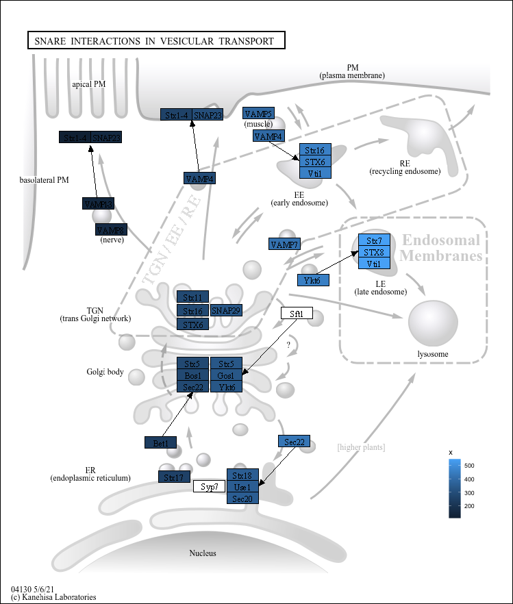

The legend outside the main panel (with_legend_image=TRUE).

g <- pathway("hsa04130")
gg <- ggraph(g, layout="manual", x=x, y=y)+
    geom_node_rect(aes(fill1=x, filter=type=="gene"))+
    geom_node_rect(aes(fill2=y, xmin=xmin+width/2, filter=type=="gene"))+
    scale_fill_multi(aesthetics = c("fill1", "fill2"),
        name = list("Condition1", "Condition2"),
        colours = list(
            scales::brewer_pal(palette = "RdBu")(6),
            scales::brewer_pal(palette = "RdPu")(6)),
            guide = guide_colorbar(barheight = unit(50, "pt")))+
    theme_void()
output_overlay_image(gg, use_cache=TRUE, with_legend_image=TRUE, out="test3.png")
#> [1] "test3.png"

knitr::include_graphics("test3.png")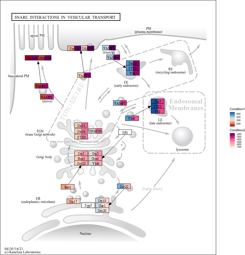

Using high resolution (2x) images (should multiply the x* and y* positions, and adjust high res parameter and legend_space parameters in output_overlay_image):

g <- pathway("hsa04130")
gg <- ggraph(g, layout="manual", x=x, y=y)+
    geom_node_rect(aes(fill1=x, xmin=xmin*2, xmax=xmax*2, ymin=ymin*2, ymax=ymax*2, filter=type=="gene"))+
    geom_node_rect(aes(fill2=y, xmin=xmin*2+width, xmax=xmax*2, ymin=ymin*2, ymax=ymax*2, filter=type=="gene"))+
    scale_fill_multi(aesthetics = c("fill1", "fill2"),
        name = list("Condition1", "Condition2"),
        colours = list(
            scales::brewer_pal(palette = "RdBu")(6),
            scales::brewer_pal(palette = "RdPu")(6)),
            guide = guide_colorbar(barheight = unit(50, "pt")))+
    theme_void()
output_overlay_image(gg, high_res=TRUE, use_cache=TRUE, with_legend_image=TRUE,
    res=100, legend_space=100,
    out="test4.png")
#> [1] "test4.png"

knitr::include_graphics("test4.png")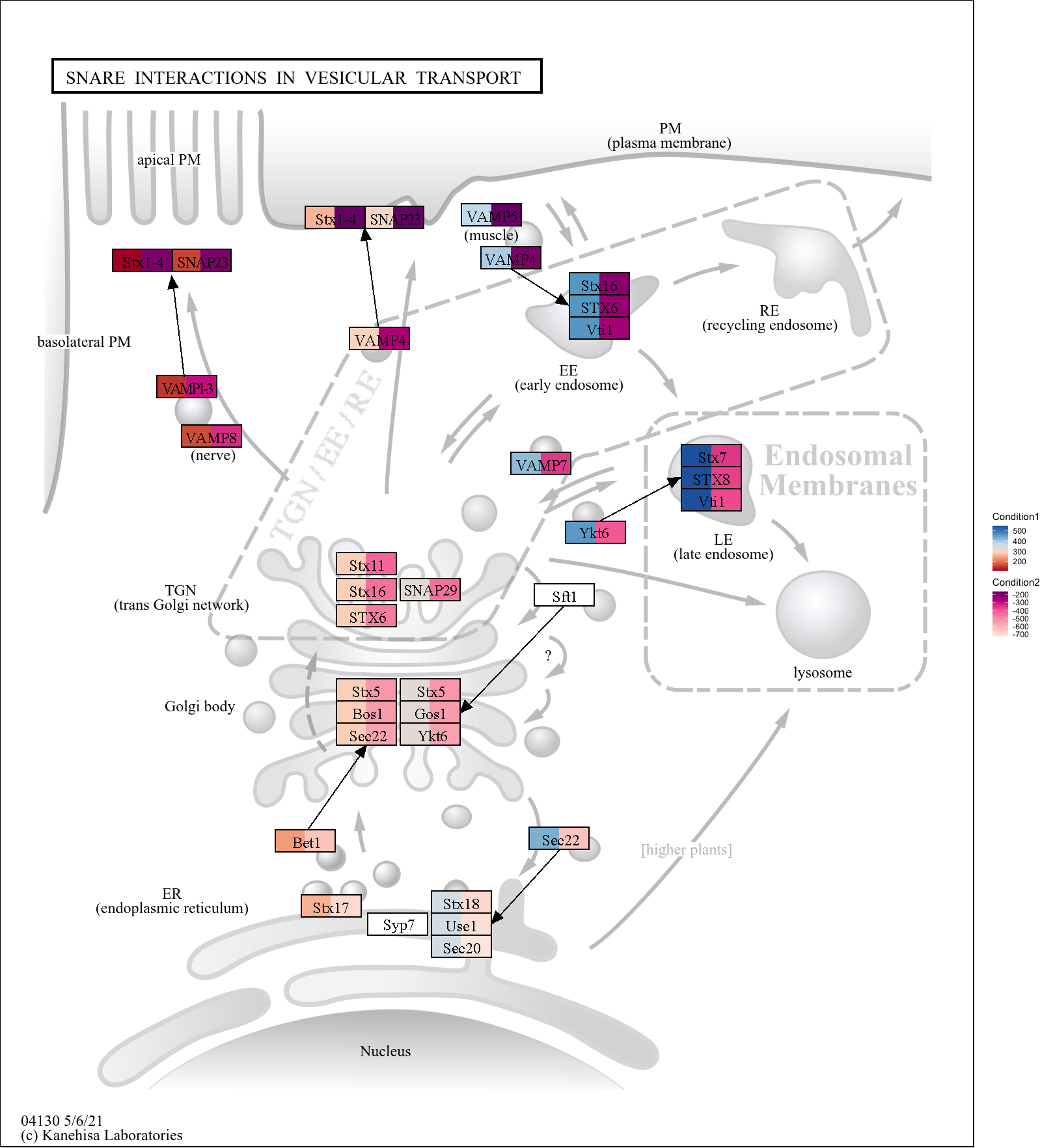

This makes sure the original image resolution is preserved.