2 Pathway
Providing ggkegg a pathway ID, it fetches information, parse them and make ggraph object. Inside, parse_kgml or pathway function is used to return igraph or tbl_graph object. It can be used with all the pathways across organisms listed in KEGG PATHWAY database.
The pathway function is a core function that downloads and parses KGML files. If the file already exists in the current working directory, it will not be downloaded again. The function also extracts reactions that are included in the pathway as edges. If there are nodes represented by type=line, the function converts these nodes to edges based on their coords. This conversion is carried out by the process_line function.
library(ggkegg)
library(ggfx)
library(ggraph)
library(igraph)
library(clusterProfiler)
library(dplyr)
library(tidygraph)
2.1 Example visualization
This example first fetches eco00270 and parse the information, convert the pathway and eco identifiers, delete zero degree nodes and returns the igraph object. The resulting graph can be plotted by ggraph, with specifying visualization of various types of information in KEGG PATHWAY in each layer.
g <- ggkegg(pid="eco00270",
            convert_org = c("pathway","eco"),
            delete_zero_degree = TRUE,
            return_igraph = TRUE)
gg <- ggraph(g, layout="fr")
gg$data$type |> unique()
#> [1] "map"      "compound" "gene"
gg + geom_edge_diagonal(
  aes(color=subtype_name,
      filter=type!="maplink"))+
  geom_node_point(
  aes(filter= !type%in%c("map","compound")),
    fill=gg$data[!gg$data$type%in%c("map","compound"),]$bgcolor,
    color="black",
    shape=21, size=4
  )+
  geom_node_point(
    aes(filter= !type%in%c("map","gene")),
    fill=gg$data[!gg$data$type%in%c("map","gene"),]$bgcolor,
    color="black",
    shape=21, size=6
  )+
  geom_node_text(
    aes(label=converted_name,
        filter=type=="gene"),
    repel=TRUE,
    bg.colour="white")+
  theme_void()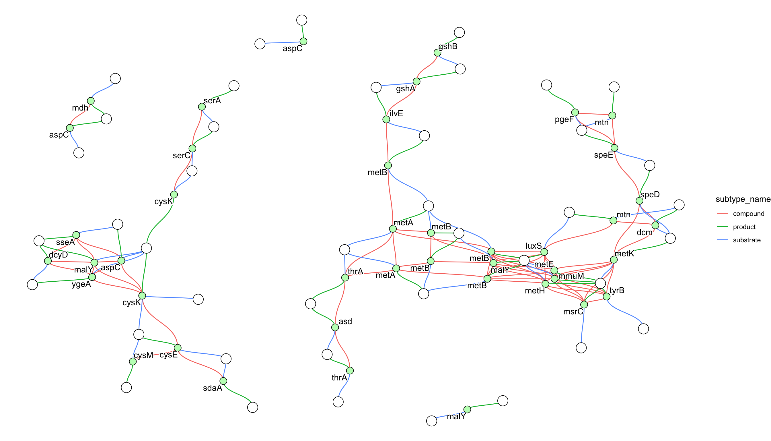
The x-coordinate, y-coordinate, width, and height described in the KGML are listed as x, y, width, and height. Based on this information, xmin, xmax, ymin, and ymax are calculated and stored in the node table.
2.2 geom_node_rect
This package also provides the geom_node_rect function, which allows drawing rectangles at specified locations based on mappings of xmin, xmax, ymin, and ymax.
2.2.1 Assigning colors to nodes
You can set diffent and multiple colors on nodes using geom_node_rect. This application is useful when visualizing factors such as log2 fold change among multiple conditions.
g <- pathway("ko00520")
V(g)$color_one <- colorRampPalette(RColorBrewer::brewer.pal(5,"Set1"))(length(V(g)))
V(g)$color_two <- colorRampPalette(RColorBrewer::brewer.pal(5,"Set2"))(length(V(g)))

ggraph(g, x=x, y=y) +
  geom_node_rect(aes(xmin=xmin, xmax=x, fill=I(color_one)), alpha=0.5)+
  geom_node_rect(aes(xmin=x, xmax=xmax, fill=I(color_two)), alpha=0.5)+
  ggfx::with_outer_glow(geom_node_text(aes(label=name |>
                       strsplit(":") |>
                       sapply("[", 2) |>
                       strsplit(" ") |>
                       sapply("[", 1),
                     filter=type=="ortholog"),
                     size=2), colour="white", expand=1)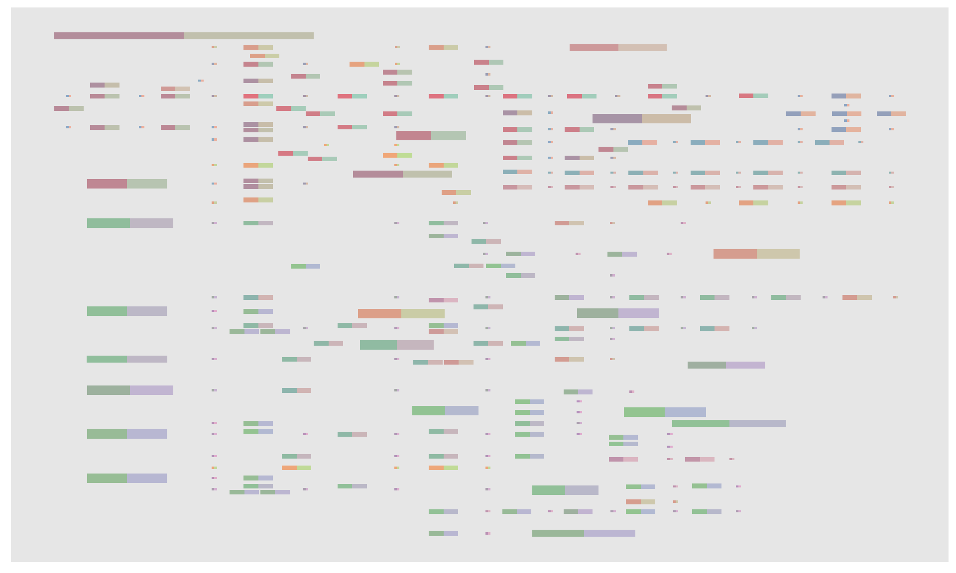
It is possible to specify any number of groups.
V(g)$color_one <- colorRampPalette(RColorBrewer::brewer.pal(5,"Set1"))(length(V(g)))
V(g)$color_two <- colorRampPalette(RColorBrewer::brewer.pal(5,"Set2"))(length(V(g)))
V(g)$color_three <- colorRampPalette(RColorBrewer::brewer.pal(5,"PuOr"))(length(V(g)))
V(g)$color_four <- colorRampPalette(RColorBrewer::brewer.pal(5,"Paired"))(length(V(g)))

V(g)$space <- V(g)$width/4

ggraph(g, x=x, y=y) +
  geom_node_rect(aes(xmin=xmin, xmax=xmin+space, fill=I(color_one), filter=type=="ortholog"))+
  geom_node_rect(aes(xmin=xmin+space, xmax=xmin+2*space, fill=I(color_two), filter=type=="ortholog"))+
  geom_node_rect(aes(xmin=xmin+2*space, xmax=xmin+3*space, fill=I(color_three), filter=type=="ortholog"))+
  geom_node_rect(aes(xmin=xmin+3*space, xmax=xmin+4*space, fill=I(color_four), filter=type=="ortholog"))+
  ggfx::with_outer_glow(geom_node_text(aes(label=name |>
                                             strsplit(":") |>
                                             sapply("[", 2) |>
                                             strsplit(" ") |>
                                             sapply("[", 1),
                                           filter=type=="ortholog"),
                                       size=2), colour="white", expand=1)+
  theme_void()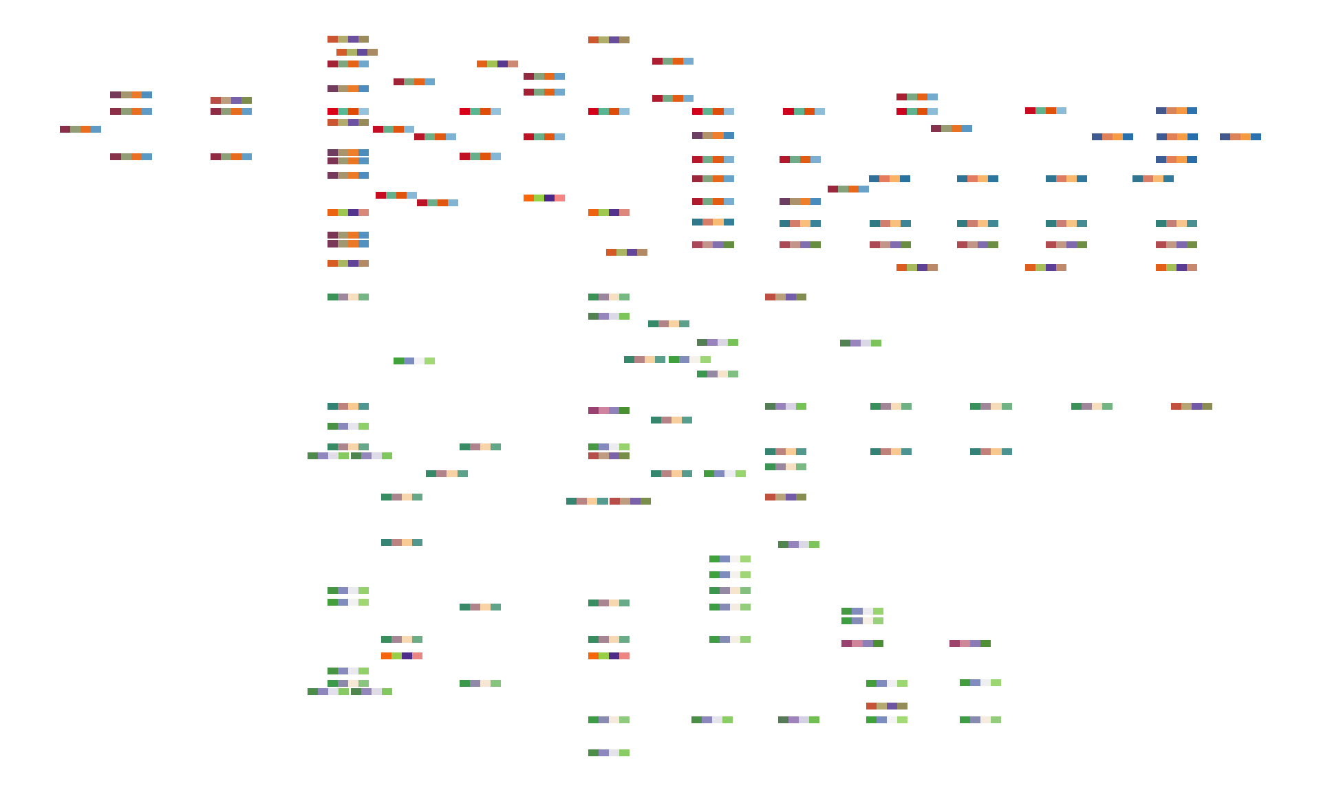
2.2.2 Multiple colors in the node data
The above visualization can be made by a function geom_node_rect_multi. This accepts the node column name specifying the color.
g %N>% filter(type=="ortholog") %>%
    ggraph(x=x, y=y) +
        geom_node_rect_multi(color_one, color_two, color_three) +
        theme_void()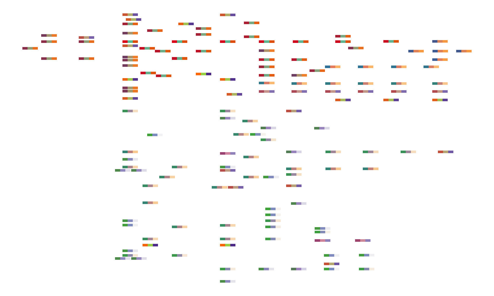
2.3 geom_node_shadowtext
Plot the shadowtext at the x and y position without enabling repel=TRUE in geom_node_text.
2.4 Global maps
For global maps, process_line function, which makes nodes and edges based on coords attributes in KGML, is prepared. However, we cannot obtain and parse directed relationship (substrate to product, reversible or irreversible) based on coords. If you would like to retain these relationships, process_reaction function is prepared.
pathway("ko01200") |>
    process_reaction() |>
    activate(nodes) |>
    mutate(x=NULL, y=NULL,
       comp=convert_id("compound")) |>
    mutate(degree=centrality_degree(mode="all")) |>
ggraph(layout="kk")+
    geom_node_point(aes(color=degree,
                        filter=type=="compound"))+
    geom_edge_parallel(
        color="grey",
        end_cap=circle(1,"mm"),
        start_cap=circle(1,"mm"),
        arrow=arrow(length=unit(1,"mm"),type="closed"))+
    geom_node_text(aes(label=comp,filter=degree>15),
                   repel=TRUE, bg.colour="white")+
    theme_graph()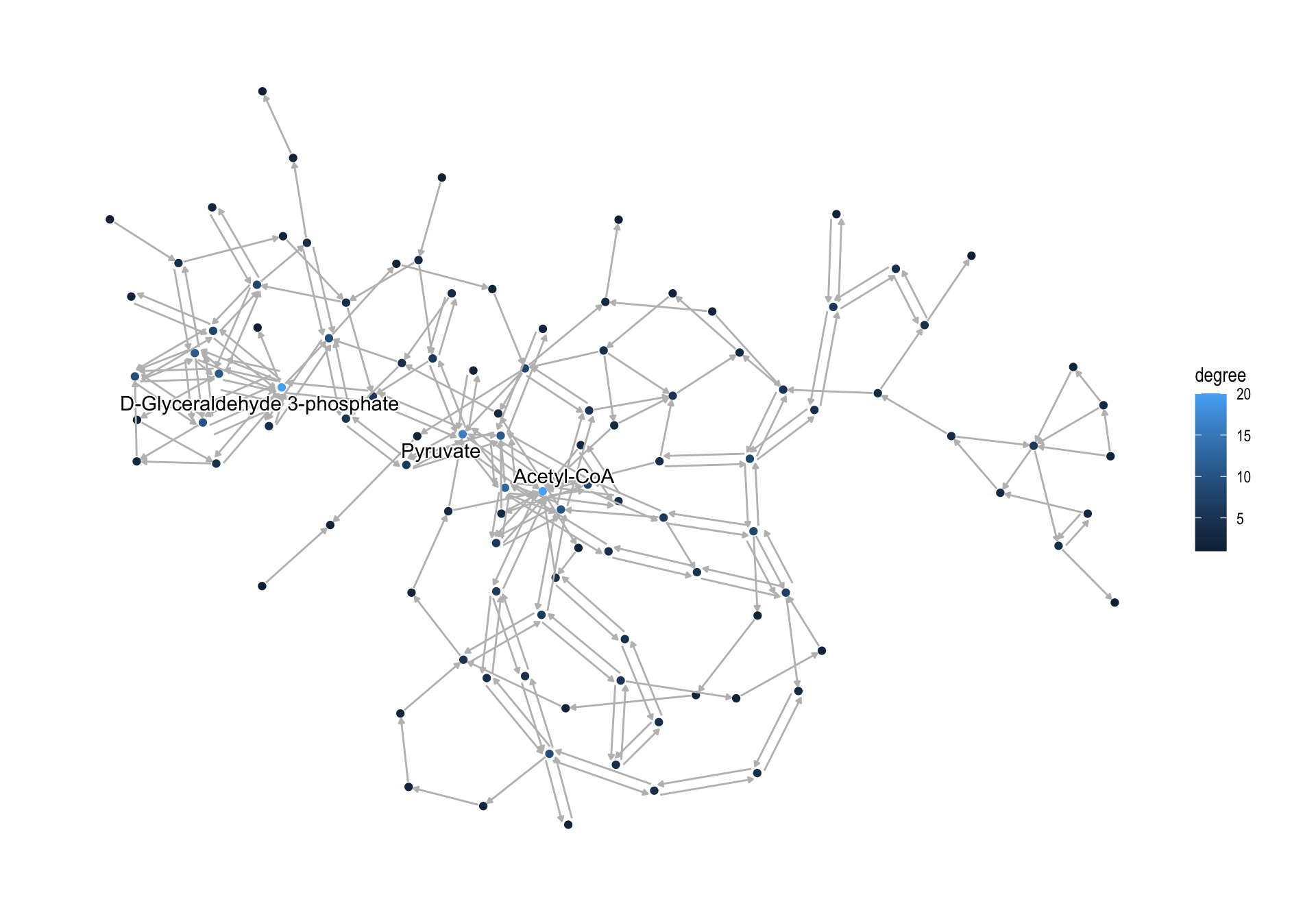
2.5 Highlighting set of nodes and edges
If you want to obtain ko01230, and highlight those components
involved in M00002, and show the corresponding compound names in the map,
we can write as follows using highligh_set_edges and highlight_set_nodes.
pathway("ko01230") |>
    process_line() |>
    activate(nodes) |>
    mutate(
        compound=convert_id("compound"),
        M00002=highlight_set_nodes(attr(module("M00002"), "reaction_components"))
    ) |>
    activate(edges) |>
    mutate(
        M00002=highlight_set_edges(attr(module("M00002"), "definition_components"))
    ) |>
    ggraph(x=x, y=y)+
        geom_edge_link()+
        with_outer_glow(
            geom_edge_link(aes(color=M00002, filter=M00002)),
        colour="pink")+
        geom_node_point(shape=21,aes(filter=type!="line"))+
        with_outer_glow(
            geom_node_point(shape=21, aes(filter=M00002, color=M00002)),
        colour="pink")+
        geom_node_text(aes(label=compound, filter=M00002), repel=TRUE,
            bg.colour="white", size=2)+
        theme_void()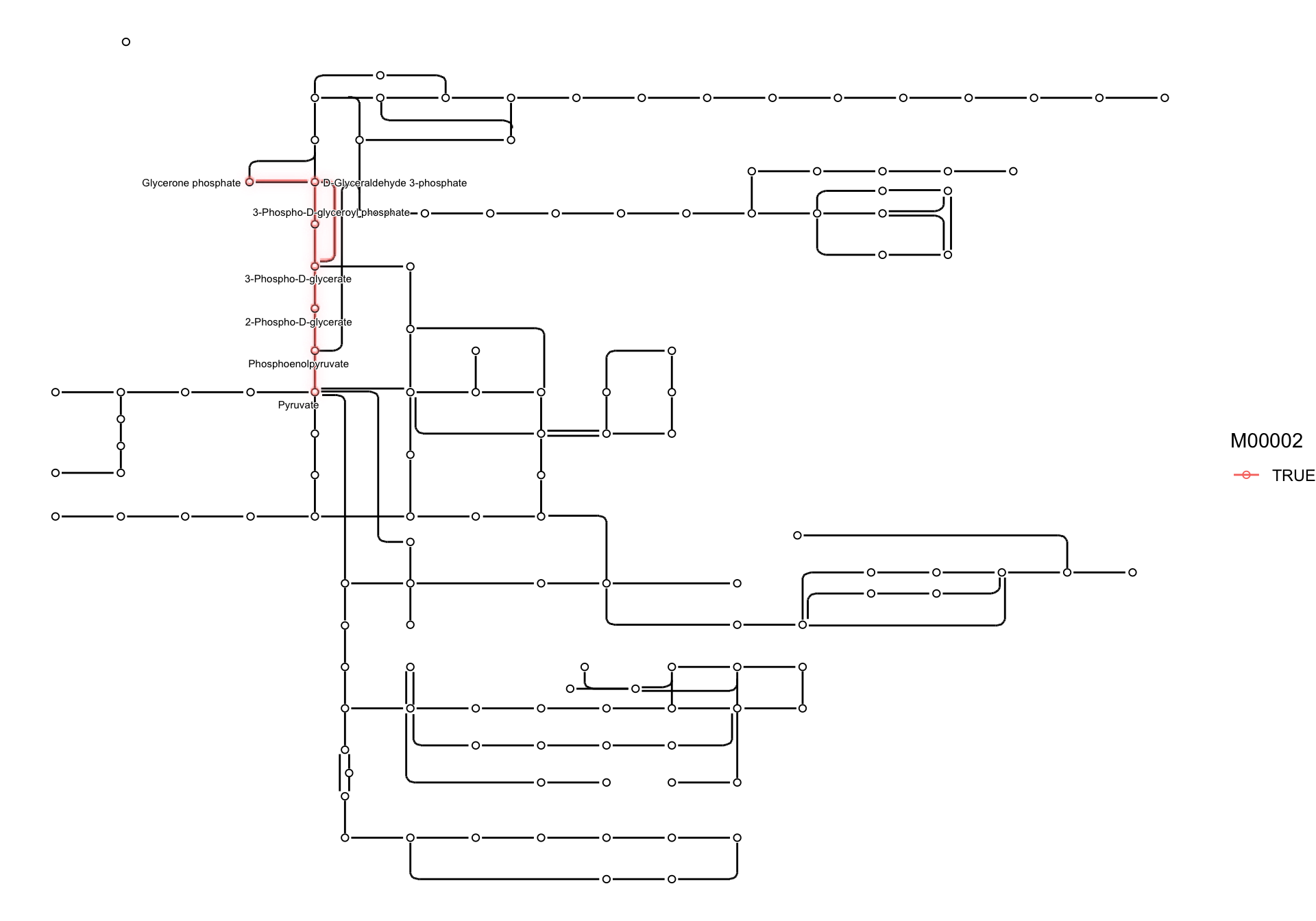
We show the example for highlighting Metabolic pathways (ko01100), using M00021 definition. highlight_module function accepts kegg_module class object and return the boolean of which edges are involved in reaction inside module and which nodes are compounds involved in the reaction. Please note that this does not produce exactly the same output as KEGG mapper. This adds new columns to the tbl_graph with TRUE for nodes and edges that meet the respective conditions.
g <- pathway("ko01100") |>
  process_line() |>
  highlight_module(module("M00021")) |>
  mutate(compound=convert_id("compound"))

g |> ggraph(x=x, y=y) +
  geom_node_point(size=1, aes(color=I(fgcolor),
    filter=fgcolor!="none" & type!="line"))+
  geom_edge_link(width=0.1, aes(color=I(fgcolor),
                                filter=type=="line"& fgcolor!="none"))+
  with_outer_glow(
    geom_edge_link(width=1,
                   aes(color=I(fgcolor),
                       filter=fgcolor!="none" & M00021)),
    colour="red", expand=3
  )+
  with_outer_glow(
    geom_node_point(size=2,
                   aes(color=I(fgcolor),
                       filter=fgcolor!="none" & M00021)),
    colour="red", expand=3
  )+
  theme_void()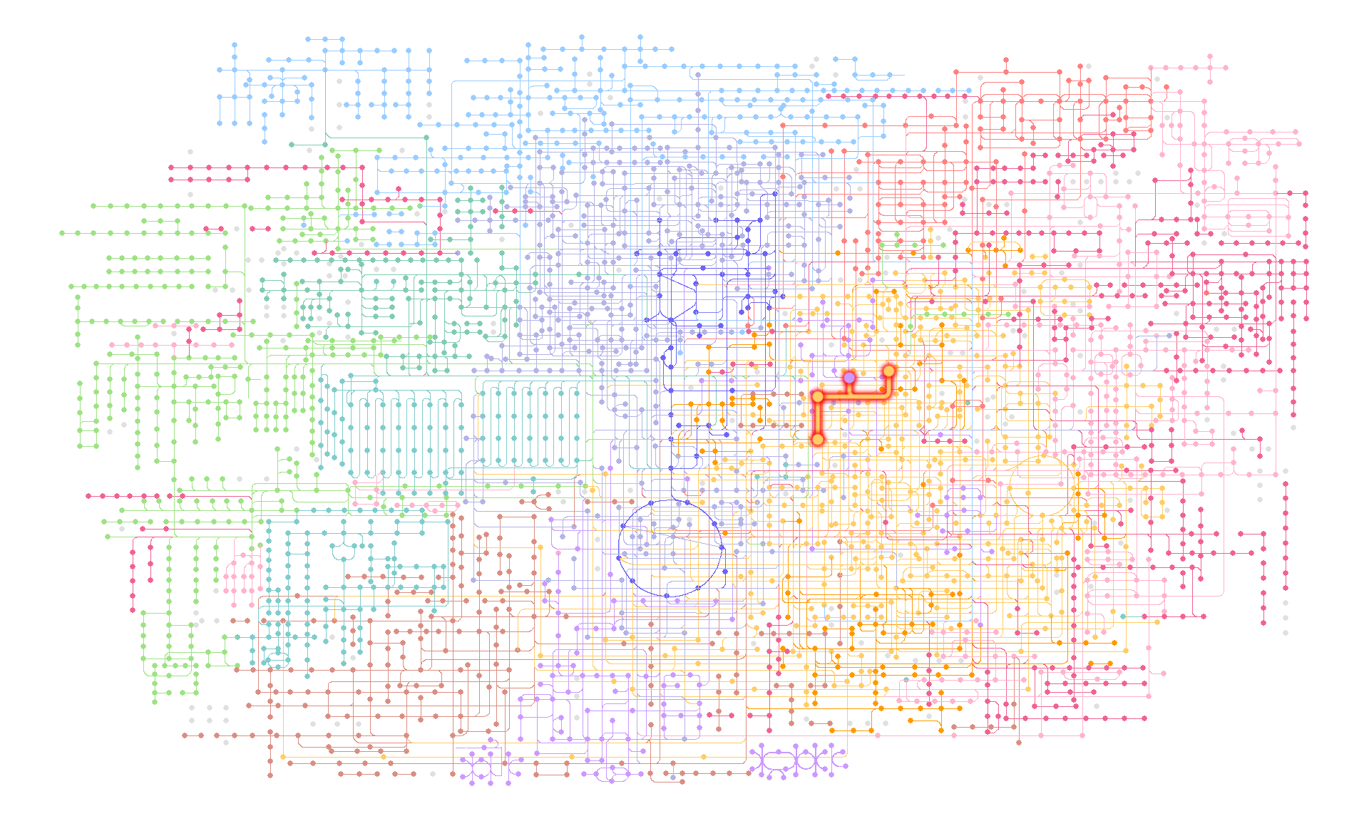
Multiple modules involved in Cysteine and methionine metabolism, highlighting M00017 by ggforce.
list_of_modules <- c("M00021","M00338","M00609","M00017","M00034","M00035","M00368")
for (mm in list_of_modules) {
  g <- g |> highlight_module(module(mm))
}

ggraph(g,x=x,y=y,layout="manual") +
  geom_edge_link0(width=0.5, color="grey")+
  geom_edge_link(color="red",aes(filter=M00017|M00021|M00338|M00609|M00034|M00035|M00368))+
geom_node_point(size=2, color="red",aes(filter=M00017|M00021|M00338|M00609|M00034|M00035|M00368))+
  ggforce::geom_mark_rect(aes(fill=M00017,
                              label=attr(module("M00017"), "name"),
                              x=x, y=y,
                              group=M00017,
                              filter=M00017),
                          label.fill = "transparent",
                          label.fontsize = 10,
                          expand=unit(1,"mm"))+
  theme_void()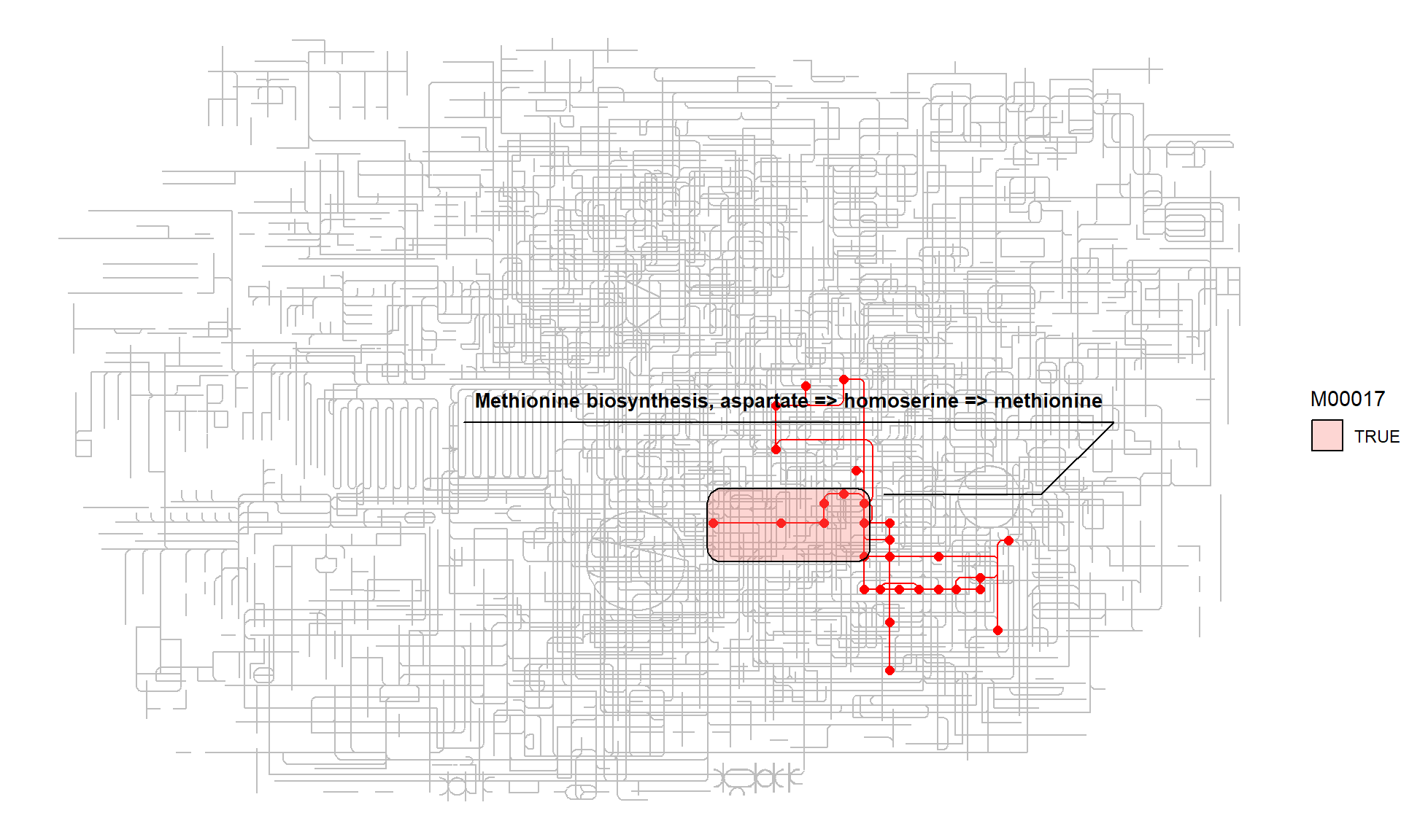
When visualizing information about compounds, it is recommended to use geom_node_text, ggrepel, and shadowtext.
g |> ggraph(x=x, y=y) +
  geom_node_point(size=1, aes(color=I(fgcolor),
    filter=fgcolor!="none" & type!="line"))+
  geom_edge_link(width=0.1, aes(color=I(fgcolor),
                                filter=type=="line"& fgcolor!="none"))+
  with_outer_glow(
    geom_edge_link(width=1,
                   aes(color=I(fgcolor),
                       filter=fgcolor!="none" & M00021)),
    colour="red", expand=3
  )+
  with_outer_glow(
    geom_node_point(size=2,
                   aes(color=I(fgcolor),
                       filter=fgcolor!="none" & M00021)),
    colour="red", expand=3
  )+
    geom_node_text(aes(label=compound, filter=M00021),
                   repel=TRUE, bg.colour="white", size=5)+
  theme_void()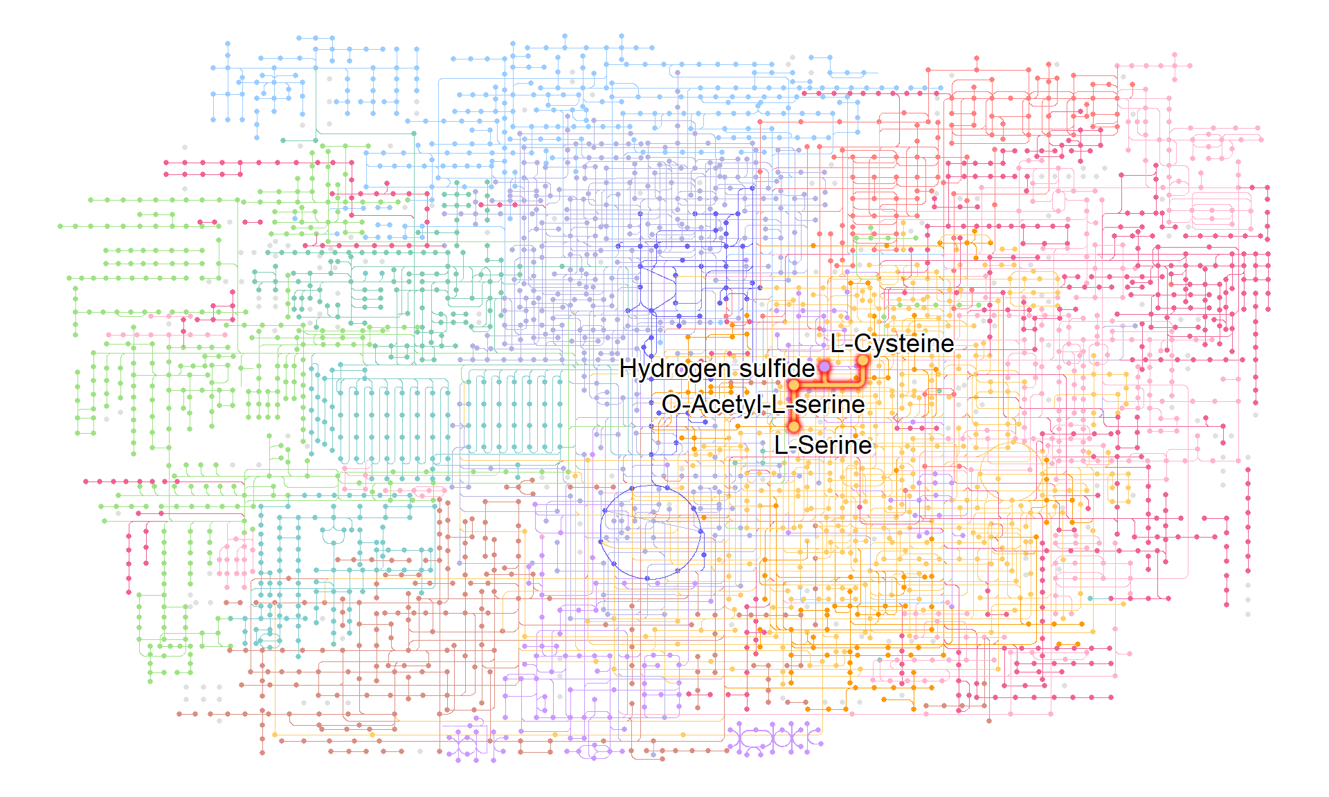
If necessary, it is possible to visualize what information is included in the highlighted pathway and place it on the original map using the annotation_custom function. In this example, an annotation ggplot is first created and then converted to a grob using ggplotify. The grob is then drawn at any desired position.
annot <- g |>  ggraph(x=x, y=y)+
  with_outer_glow(
    geom_edge_link(width=1,
                   aes(color=I(fgcolor),
                       filter=fgcolor!="none" & M00021)),
    colour="red", expand=3
  )+
  with_outer_glow(
    geom_node_point(size=2,
                    aes(color=I(fgcolor),
                        filter=fgcolor!="none" & M00021)),
    colour="red", expand=3
  )+
    geom_node_text(aes(label=compound, filter=M00021),
                   repel=TRUE, bg.colour="white", size=5)
g |>
  ggraph(x=x, y=y) +
  geom_node_point(size=1, aes(color=I(fgcolor),
                              filter=fgcolor!="none" & type!="line"))+
  geom_edge_link(width=0.1, aes(color=I(fgcolor),
                                filter=type=="line"& fgcolor!="none"))+
  with_outer_glow(
    geom_edge_link(width=1,
                   aes(color=I(fgcolor),
                       filter=fgcolor!="none" & M00021)),
    colour="red", expand=3
  )+
  with_outer_glow(
    geom_node_point(size=2,
                    aes(color=I(fgcolor),
                        filter=fgcolor!="none" & M00021)),
    colour="red", expand=3
  )+
  annotation_custom(ggplotify::as.grob(annot),
    ymin=-1500, ymax=0, xmin=0, xmax=1500)+ ## your desired position
  theme_void()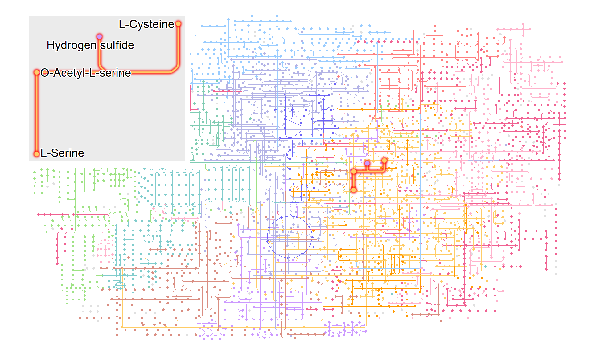
It is also possible to highlight any desired edges or nodes. In this case, the highlight_set_edges and highlight_set_nodes functions are used within mutate to generate a new column containing a boolean indicating whether the specified IDs are included or not. We can highlight those nodes or edges in the desired geoms. When how is set to all, TRUE is returned only if all the IDs included in the query are included in the node. When how is set to any, TRUE is returned if any of the IDs included in the query are included in the node.
gg <- g |> activate(edges) |>
  mutate(highlight=highlight_set_edges(c("ko:K00790","ko:K00789")))
gg |>
  ggraph(x=x, y=y) + geom_edge_link(width=0.1, aes(filter=fgcolor!="none",
                                                   color=I(fgcolor))) +
  with_outer_glow(geom_edge_link(width=1, aes(filter=highlight,
   color=I(fgcolor))), colour="red", expand=3) + theme_graph()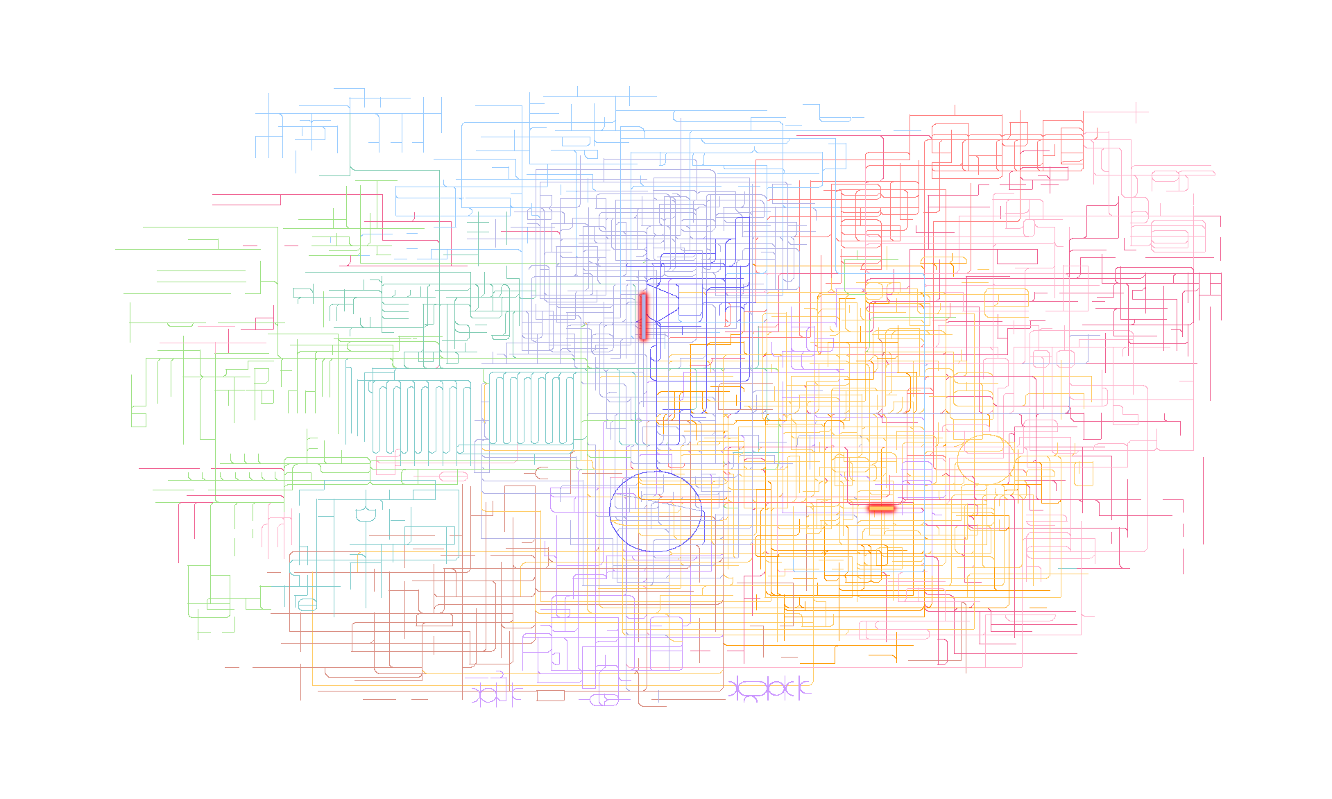
An example of highlighting combined with the graphhighlight:
library(graphhighlight)
g |> ggraph(x=x, y=y) +
  geom_edge_link(width=0.5, aes(color=I(fgcolor), filter=fgcolor!="none")) +
  geom_node_point(size=1, aes(color=I(fgcolor), filter=fgcolor!="none" & type!="line"))+
  highlight_node(glow=TRUE, filter=fgcolor!='none' & type!='line',
                 glow_base_size=TRUE,glow_size=0.5)+
  theme_void()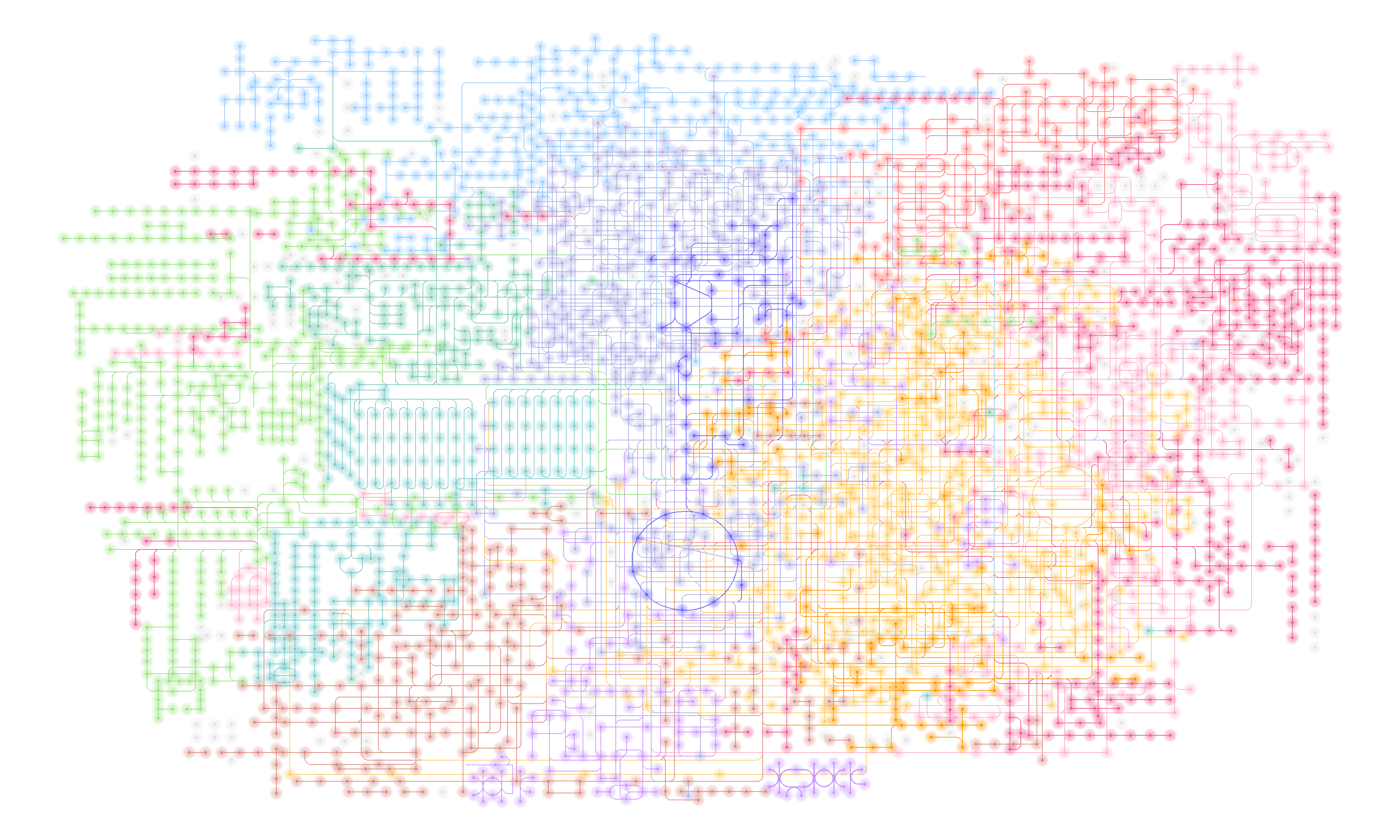
When visualizing large maps such as global and overview maps, it is better to use geom_edge_link0, as described in the documentation of ggraph geom_edge_*. Moreover, for nodes, combining the scattermore package’s geom_scattermore with ggraph’s StatFilter allows for faster rendering.
st <- Sys.time()
ggraph(g, x=x, y=y) +geom_edge_link0(aes(color=I(fgcolor)))+
  scattermore::geom_scattermore(pointsize=1, stat=StatFilter,
    aes(x=x, y=y, color=I(fgcolor),
    filter=type!="map"))+theme_void()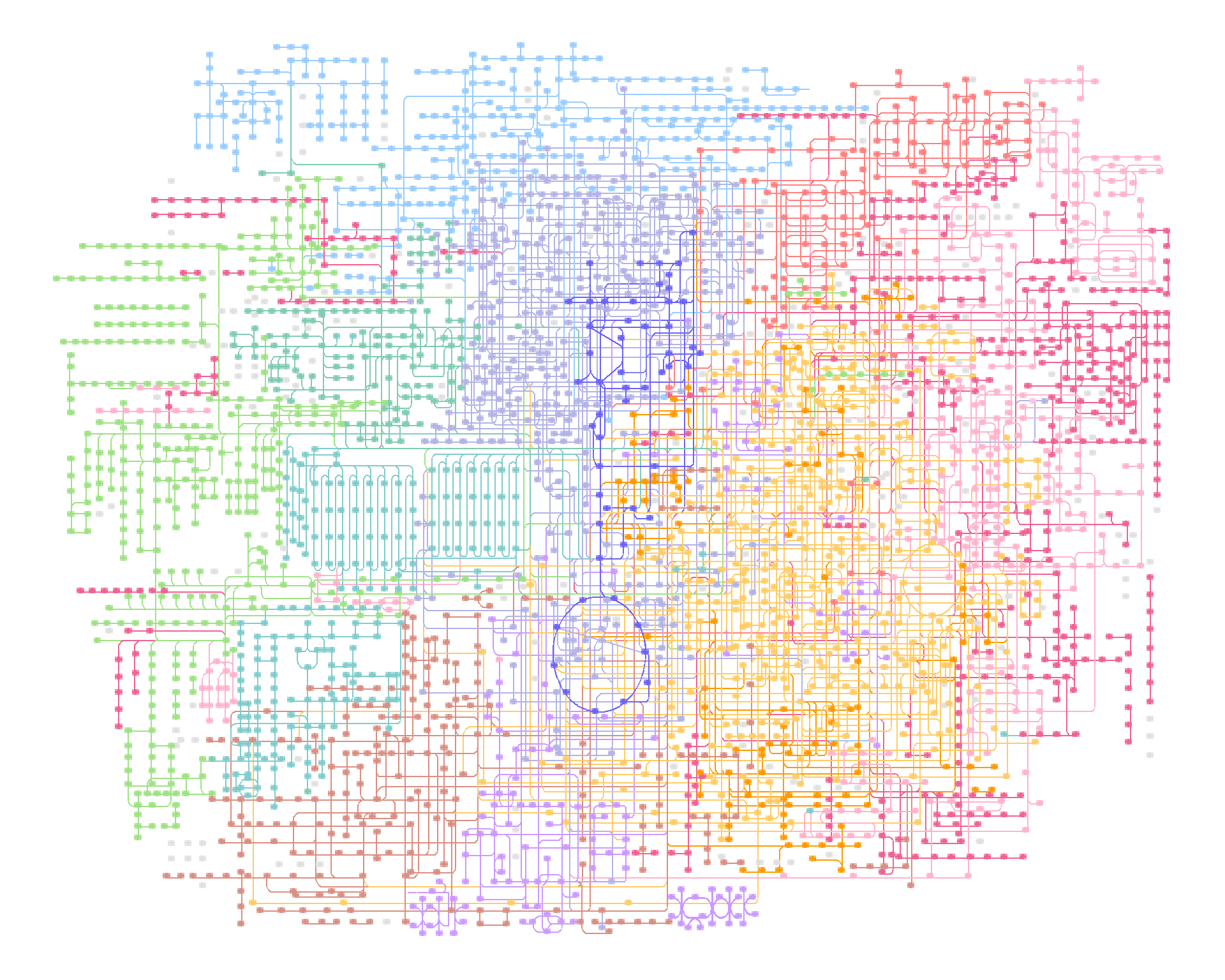
ed <- Sys.time()
ed-st
#> Time difference of 1.296499 secs

st <- Sys.time()
ggraph(g, x=x, y=y) +geom_edge_link(aes(color=I(fgcolor)))+
  geom_node_point(size=2, aes(color=I(fgcolor),
    filter=type!="map"))+theme_void()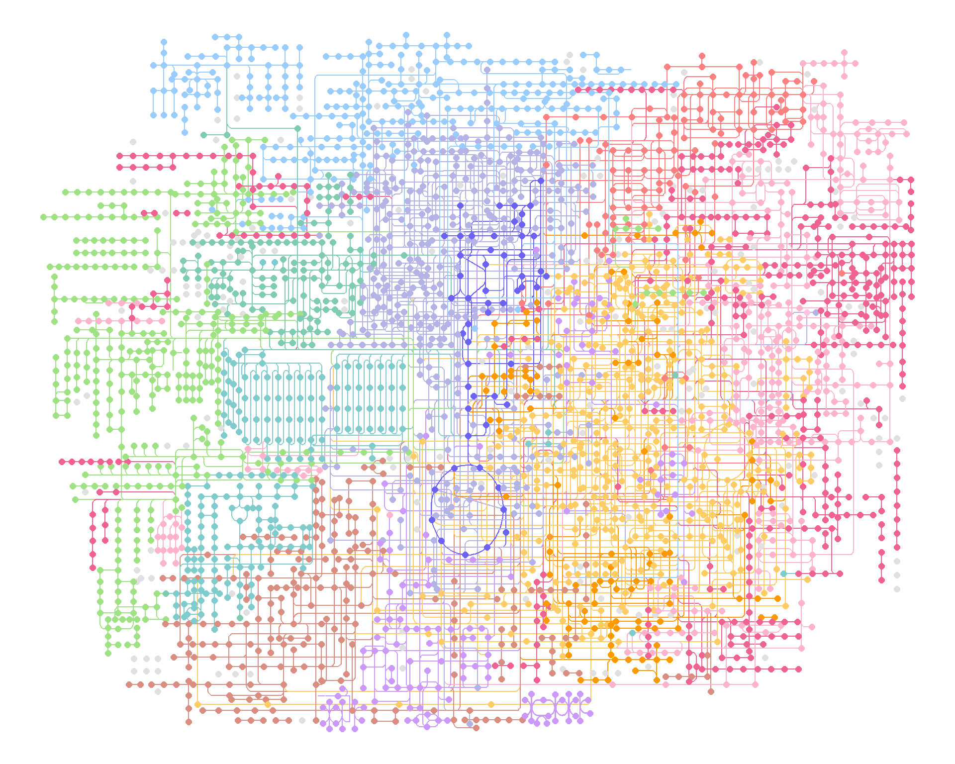
ed <- Sys.time()
ed-st
#> Time difference of 48.93137 secs
2.6 Overlaying original KEGG pathway images on ggraph
Using magick, you can overlay the original KEGG pathway image on the graph you made (or add components on the original image). The package provides overlay_raw_map function, which allows mapping a raster image onto the graph by specifying the pathway ID and the color to be made transparent.
g <- pathway("ko00640",group_rect_nudge=0) ## Obtain pathway graph (don't show grouping rect)
gg <- ggraph(g, layout="manual", x=x, y=y)+
  geom_node_point(aes(filter=type=="compound"), color="blue", size=2)+
  geom_node_rect(fill="red",aes(filter=type=="ortholog"))+
  overlay_raw_map("ko00640")+
  theme_void()
gg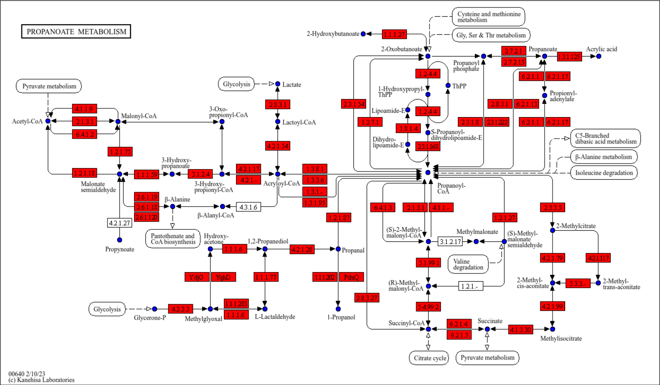
You can use your favorite geoms to annotate KEGG map combining the functions.
m <- module("M00013")
reactions_in_module <- attr(m, "reaction_components")
g <- g |> mutate(mod=highlight_set_nodes(reactions_in_module, how="all"))
gg <- ggraph(g, layout="manual", x=x, y=y)+
    geom_node_rect(fill="grey",aes(filter=type=="ortholog"))+
    geom_node_point(aes(filter=type=="compound"), color="blue", size=2)+
    overlay_raw_map("ko00640")+
    ggfx::with_outer_glow(
        geom_node_point(aes(filter=mod, x=x, y=y), color="red",size=2),
    colour="yellow",expand=5)+
    theme_void()
gg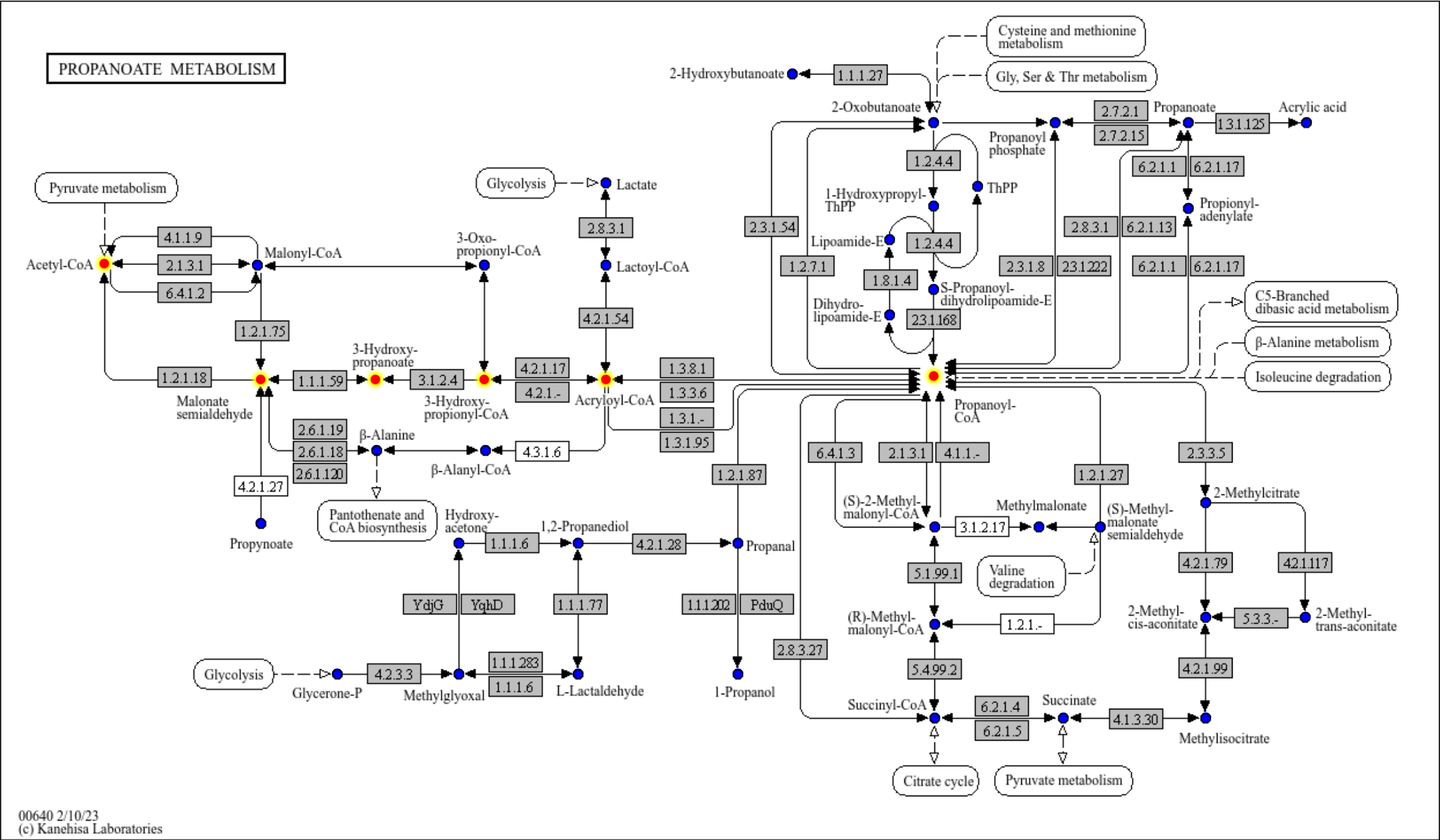
Text can be overridden by specifying rectangular geom after the raw map.
## Use graphics_name but show only the first ID
g <- pathway("ko00640",group_rect_nudge=0)
gg <- ggraph(g, layout="manual", x=x, y=y)+
  overlay_raw_map()+
  geom_node_rect(fill="white",aes(filter=type=="ortholog"), color="black")+
  geom_node_text(aes(
      label=graphics_name %>% strsplit(",") %>% sapply("[", 1) %>% strsplit("\\.") %>% sapply("[", 1),
      filter=type=="ortholog"),size=2)+
  theme_void()
gg
The reference pathway image have a version with higher resolution provided by KEGG REST API. The image can be used by enabling the high_res option in overlay_raw_map which is disabled by default. In this case, you must adjust the position of xmin, ymin, xmax and ymax by the multiplication by 2 for geom_node_rect and x and y for geom_node_text.
g <- pathway("ko00640")
gg <- ggraph(g, layout="manual", x=x*2, y=y*2)+
  overlay_raw_map(high_res=TRUE)+
  geom_node_rect(fill="white",
      aes(xmin=xmin*2, xmax=xmax*2, ymin=ymin*2, ymax=ymax*2, filter=type=="ortholog"), color="black")+
  geom_node_text(aes(
      label=graphics_name %>% strsplit(",") %>% sapply("[", 1) %>% strsplit("\\.") %>% sapply("[", 1),
      filter=type=="ortholog"),size=4)+
  theme_void()
gg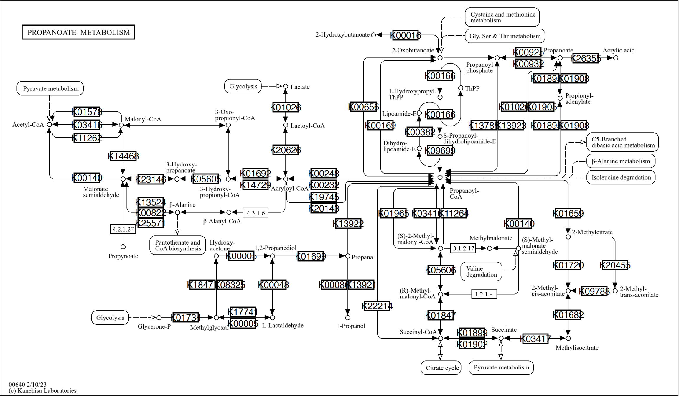
2.7 Group of nodes
The groups are specified in the KGML with type=“group”. The pathway function adds edges linking the group ID and component ID, allowing the visualization of groups in the layout other than those specified in the KGML. The edges mentioned are specified with the type in_group.
g <- pathway("hsa03460") |> mutate(conv=convert_id("hsa"))
g <- delete_vertex_attr(g, "x")
g <- delete_vertex_attr(g, "y")
ggraph(g, layout = "nicely") +
  geom_node_point(aes(filter=type=="gene" | type=="group"), color="black") +
  geom_edge_link(aes(color=subtype_name),end_cap=circle(2,"mm"),
                 start_cap=circle(2,"mm"),
                     label_dodge = unit(2,"mm"))+
  geom_node_text(aes(label=conv), repel=TRUE, bg.colour="white")+
  theme_void()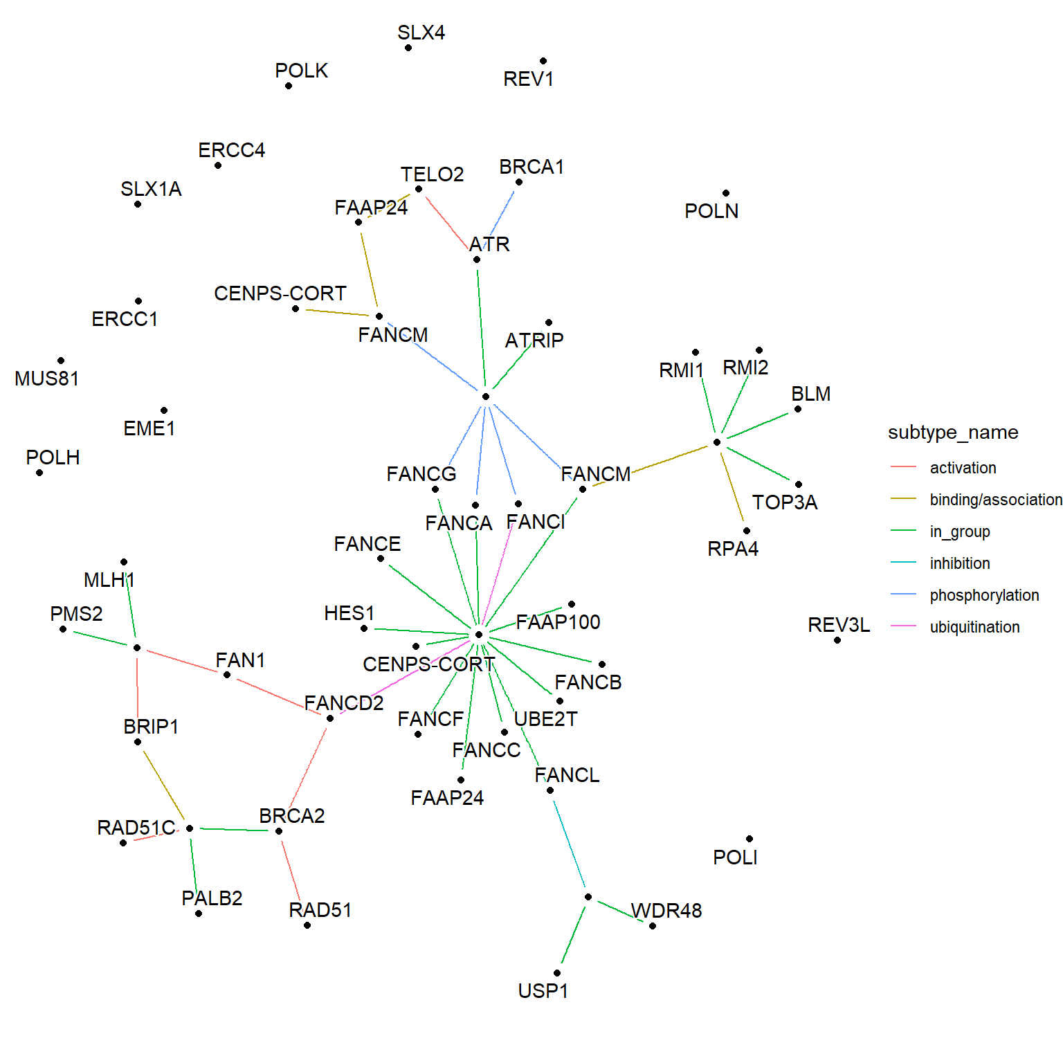
2.8 Combining multiple pathways in their native layouts
Combining multiple pathways using their native layouts is possible by mutating the nodes’ positions or contracting multiple graphs.
## Mutate X position for the first graph
g1 <-pathway("ko00640")
pos <- g1 |> activate(nodes) |> data.frame() |> summarise(min=min(y))
g1_mut <- g1 |> activate(nodes) |> mutate(x=x/max(x))

## Mutate Y position and x position for the second graph
g2 <-pathway("ko00620")
g2_mut <- g2 |> activate(nodes) |> mutate(y=y+pos$min, x=x/max(x))
joined_raw <- graph_join(g1_mut, g2_mut)
joined_name <- graph_join(g1_mut, g2_mut, by=c("name","x","y"))

## Group by node names and take attribute of first rows
## For edges, combine reaction
newg <- joined_raw |>
  convert(to_contracted, name) |>
  activate(nodes) |>
  mutate(purrr::map_vec(.orig_data, function(x) x[1,]))|>
  activate(edges) |>
  mutate(reaction=purrr::map_vec(.orig_data,
                                 function(x) paste0(unique(x$reaction),
                                                    collapse=",")),
         subtype_name=purrr::map_vec(.orig_data,
                                 function(x) unique(x$subtype_name)))
## Highlight the cpd:C00024 node for normal-joined, and contracted graph by name
## Blue color indicates occurrence in both pathway

## Normal joined
joined_name |> morph(to_contracted, name) |>
  activate(nodes) |>
  mutate(occ=purrr::map_vec(.orig_data, function(x) dim(x)[1])) |>
  unmorph() |>
  ggraph(layout="manual", x=x, y=y) +
  geom_edge_link0(width=0.1, aes(color=subtype_name,
                                 filter=subtype_name %in% c("substrate","product")))+
  geom_node_point() +
  geom_node_point(color="blue", aes(filter=occ>1))+
  graphhighlight::highlight_node(filter=name=="cpd:C00024", glow=TRUE,
                                 highlight_color = "red")+
  theme_void()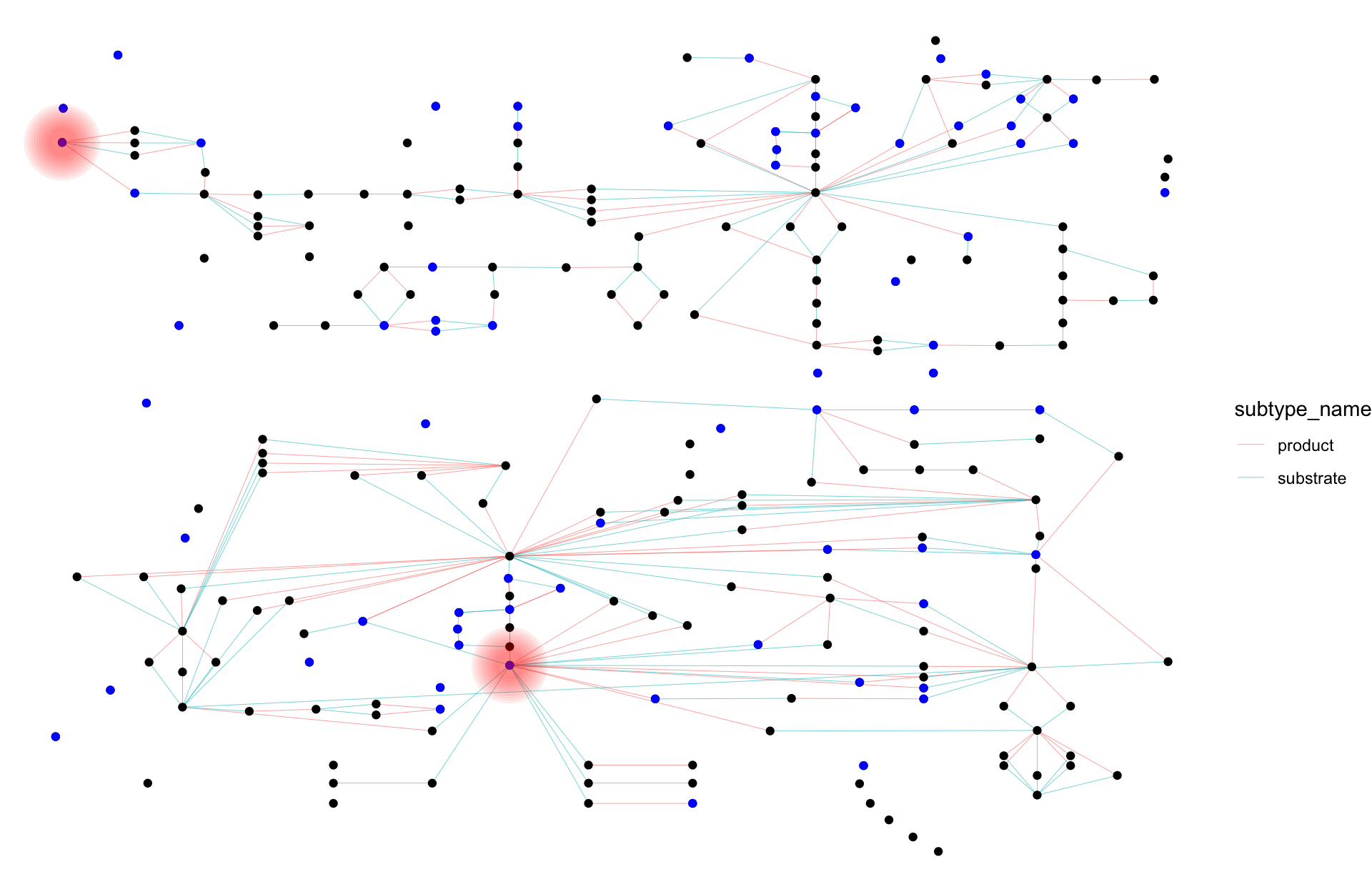
## Contracted
newg |>
  activate(nodes) |> mutate(
    ko=convert_id("ko"),
    occ=purrr::map_vec(.orig_data, function(x) dim(x)[1])) |>
ggraph(layout="manual", x=x, y=y) +
  geom_edge_link0(width=0.1, aes(color=subtype_name,
                                 filter=subtype_name %in% c("substrate","product")))+
  geom_node_point()+
  geom_node_point(color="blue", aes(filter=occ>1)) +
  geom_node_point(color="red", aes(filter=name=="cpd:C00024"))+
  graphhighlight::highlight_node(filter=name=="cpd:C00024", glow=TRUE,
                                 highlight_color = "red")+
  geom_node_text(size=1.5, family="serif", repel=TRUE, bg.colour="white",
                 aes(label=ko, filter=type=="ortholog"))+
  theme_void()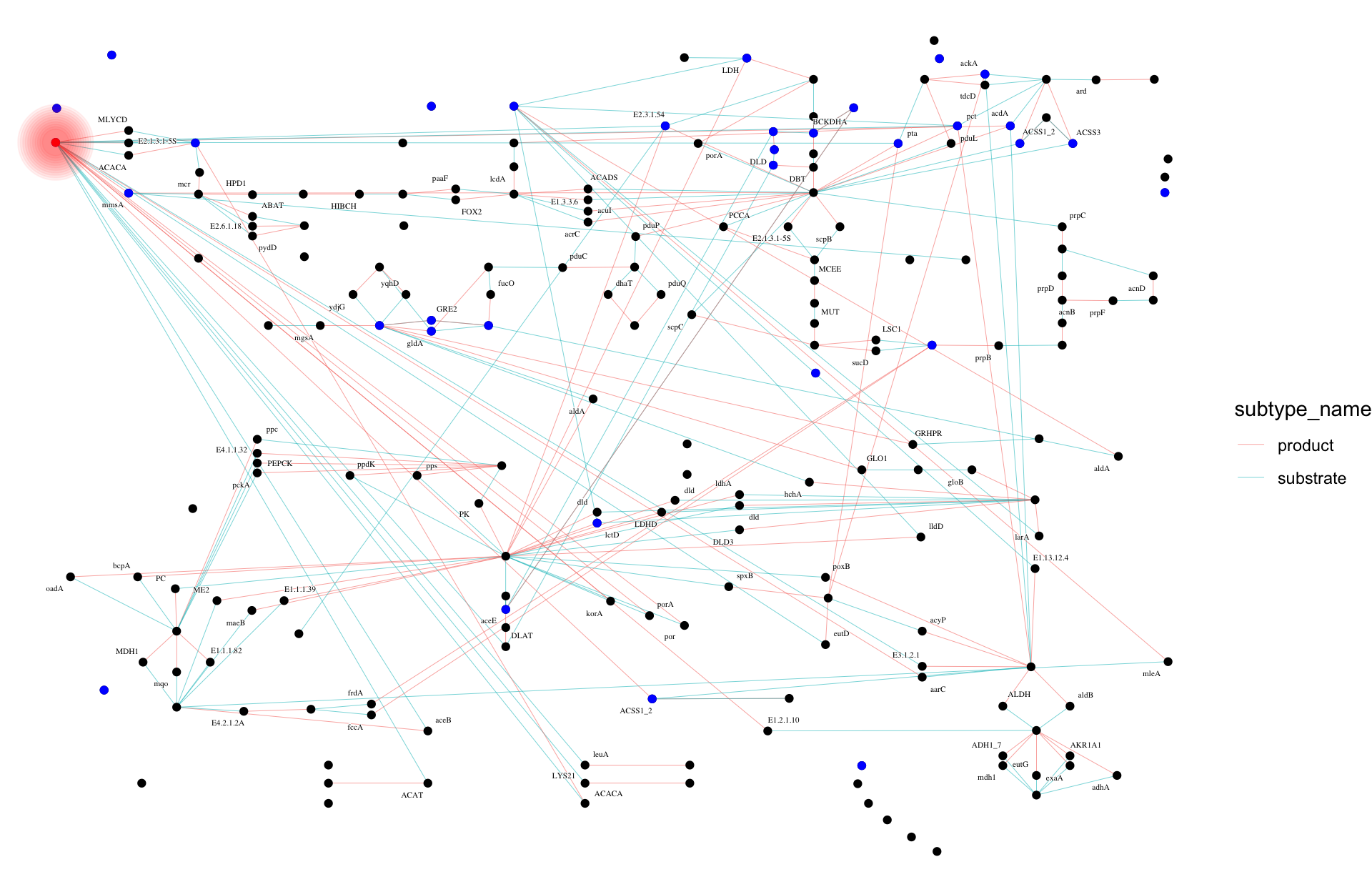
2.8.1 multi_pathway_native
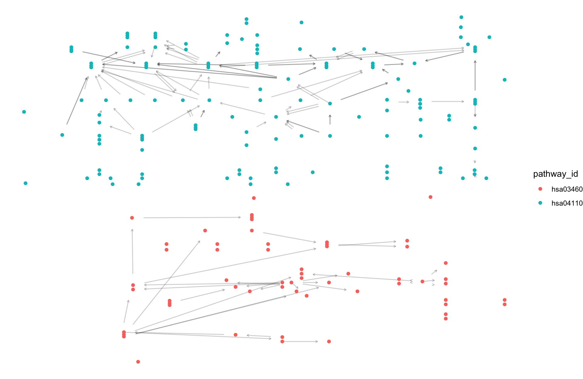
By employing the multi_pathway_native function, one can array multiple native KGML layouts on a panel. In conjunction with to_contracted, it becomes feasible to examine the relationships of genes across various pathways.
pathways <- c("hsa04110","hsa03460")
multig <- multi_pathway_native(pathways, row_num=2)

multig |>
  ggraph(layout="manual", x=x, y=y)+
  geom_edge_parallel(alpha=0.2,
                 arrow=arrow(length=unit(1,"mm")),
                 start_cap=circle(5,"mm"),
                 end_cap=circle(5,"mm"))+
  geom_node_point(aes(color=pathway_id))+
  theme_void()