Chapter 6 The other options

6.1 Bootstrap reasoning

For the bootstrapping approach, the averaged network sometimes does not hold directed acyclic assumptions, and the probabilistic reasoning cannot be performed. The bootReason function is implemented that performs probabilistic reasoning for each bootstrap replicate and return the mean of events, as well as difference in mean from the control level.

metadata <- data.frame(tcgaData@colData) %>%
  dplyr::select(age_at_diagnosis, gender, paper_mutation.in.TP53, paper_Combined.T.and.LN.category) %>% na.omit() %>%
  filter(paper_mutation.in.TP53!="ND") %>%
  filter(paper_Combined.T.and.LN.category!="ND")

## Set TP53 status to numeric of 0/1.
metadata$paper_mutation.in.TP53 <- as.numeric(as.factor(metadata$paper_mutation.in.TP53))-1
metadata$age_at_diagnosis <- as.numeric(scale(metadata$age_at_diagnosis))
metadata$paper_Combined.T.and.LN.category <- as.factor(metadata$paper_Combined.T.and.LN.category)
metadata$gender <- as.factor(metadata$gender)

## Return only the data frame
df <- bngeneplot(pway, vstedTCGA, pathNum=3, expSample=rownames(metadata),
                otherVar=metadata, otherVarName=c("Age","Gender","TP53","Category"), onlyDf=T)

## Calculate for multiple levels
tp53Res <- bootReasonOne(df, 20, node=c("CENPH","NUP107"), c("TP53"), level=c(0, 0.25, 0.5, 0.75, 1), cont=0)
kable(tp53Res$difMean)

Mean	stdev	level	node
0.0725425	0.0115887	0.25	CENPH
0.1448624	0.0218349	0.50	CENPH
0.2162356	0.0294590	0.75	CENPH
0.2854647	0.0372784	1.00	CENPH
-0.0356490	0.0192726	0.25	NUP107
-0.0630656	0.0345684	0.50	NUP107
-0.0985853	0.0524808	0.75	NUP107
-0.1296113	0.0703502	1.00	NUP107

6.2 Discretization

If passed an option disc=TRUE, the continuous variables are discretized using arules::discretize function (Hahsler et al. 2011). The discretization of the gene expression data is discussed in Gallo et al. (2016). If the same discretization is to be applied on the other data like the training and test dataset, you can pass the training samples to tr option, and if some variables are not intended to be discretized, you should pass the column name to remainCont.

bngeneplot(results = pway, exp = vsted, pathNum = 1, disc=TRUE, layout="sugiyama")

6.3 Custom visualization

6.3.1 The glowing nodes and edges

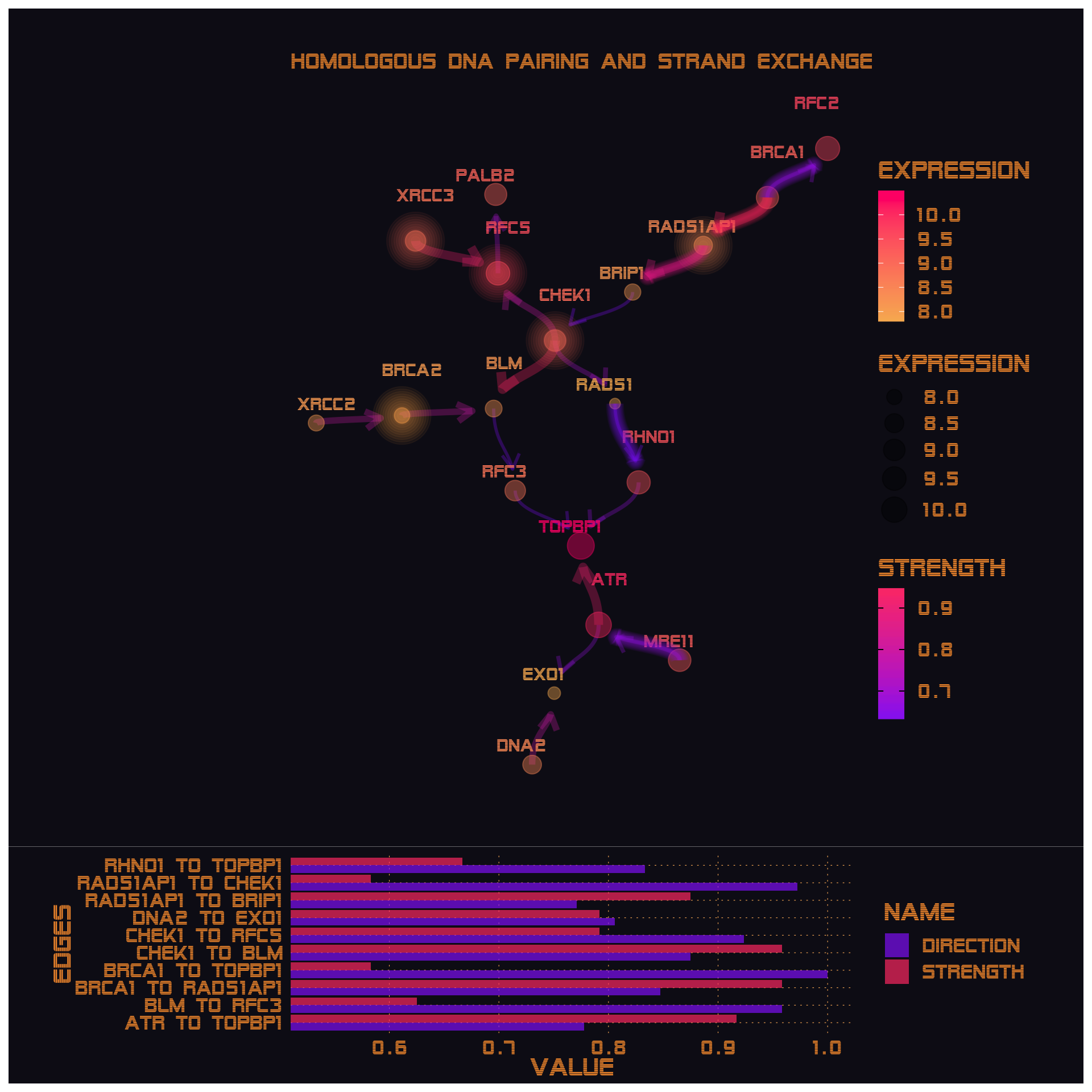
In addition to the normal plot, custom function of visualization is implemented (bngeneplotCustom and bnpathplotCustom). For example, to effectively visualize the hub genes and edges with high strength by glowing the respective nodes and edges, below is an example using an idea of ggCyberPunk. Additionally, the edge and node colors are fully customizable.

cl = parallel::makeCluster(6)
bngeneplotCustom(results = pway,
                exp = vsted,
                expSample = incSample,
                R=50, cl=cl, layout="kk", fontFamily="sans",
                pathNum = c(11), strType="normal", sizeDep=T, dep=dep,
                showDir=T, hub=5, glowEdgeNum=5, strThresh=0.6, strengthPlot = T)

For the demonstrative purpose, using the palettes and fonts of vapoRwave and showtext, the other visualizations are possible. Note that in custom visualization, only the network plot and strength barplot are supported.

## Use alien encounter fonts (http://www.hipsthetic.com/alien-encounters-free-80s-font-family/)
sysfonts::font_add(family="alien",regular="SFAlienEncounters.ttf")
showtext::showtext_auto()
cl = parallel::makeCluster(6)
bngeneplotCustom(results = pway,
                        exp = vsted,
                        expSample = incSample,
                        R=20, cl=cl, fontFamily="alien", labelSize=4,
                        pathNum = c(15), strType="normal",
                        showDir=F, hub=5, glowEdgeNum=5, strThresh=0.6,
                        strengthPlot = T, sizeDep=F, dep=dep, layout="kk",
                        edgePal=c("#9239F6","#FF4373"),
                        nodePal=c("#F8B660","#FF0076"),
                        barLegendKeyCol="#0F0D1A",
                        textCol="#EE9537", titleCol="#EE9537",
                        backCol="#0F0D1A",
                        barAxisCol="#EE9537",
                        barTextCol="#EE9537",
                        barPal=c("#9239F6", "#FF4373"),
                        barPanelGridCol="#FFB967",
                        barBackCol="#0F0D1A",
                        titleSize=14
                        )

6.4 Comparing multi scale and standard bootstrapping

cl <- parallel::makeCluster(6)
comparePlot <- bngeneplot(results = pway,
                          exp = vsted, cl=cl, strType="normal",
                          pathNum = 15, R = 50, returnNet=T,
                          shadowText = TRUE)
comparePlotMS <- bngeneplot(results = pway,
                          exp = vsted, cl=cl, strType="ms",
                          pathNum = 15, R = 50, returnNet=T,
                          shadowText = TRUE)

kable(comparePlot$str %>%
    filter(direction>0.5) %>%
    arrange(desc(strength)) %>%
    head())

from	to	strength	direction
TOPBP1	ATR	0.9814815	0.8125000
RFC5	XRCC3	0.9629630	0.6458333
RAD51AP1	BRCA1	0.9629630	0.5879630
RFC2	ATR	0.9444444	0.5462963
CHEK1	RAD51	0.9074074	0.7949735
RAD51AP1	CHEK1	0.8518519	0.7739749

kable(comparePlotMS$str %>%
    filter(direction>0.5) %>%
    arrange(desc(strength)) %>%
    head())

from	to	strength	direction
RFC5	XRCC3	0.9988307	0.5143560
RFC2	ATR	0.9981892	0.8251665
BRIP1	BRCA2	0.9951984	0.6876182
DNA2	BLM	0.9933508	0.6871648
TOPBP1	ATR	0.9929435	0.8779386
RFC3	ATR	0.9874010	0.8598716

References

Gallo, Cristian A, Rocio L Cecchini, Jessica A Carballido, Sandra Micheletto, and Ignacio Ponzoni. 2016. “Discretization of Gene Expression Data Revised.” Brief. Bioinform. 17 (5): 758–70.

Hahsler, Michael, Sudheer Chelluboina, Kurt Hornik, and Christian Buchta. 2011. “The Arules R-Package Ecosystem: Analyzing Interesting Patterns from Large Transaction Data Sets.” J. Mach. Learn. Res. 12 (57): 2021–25.