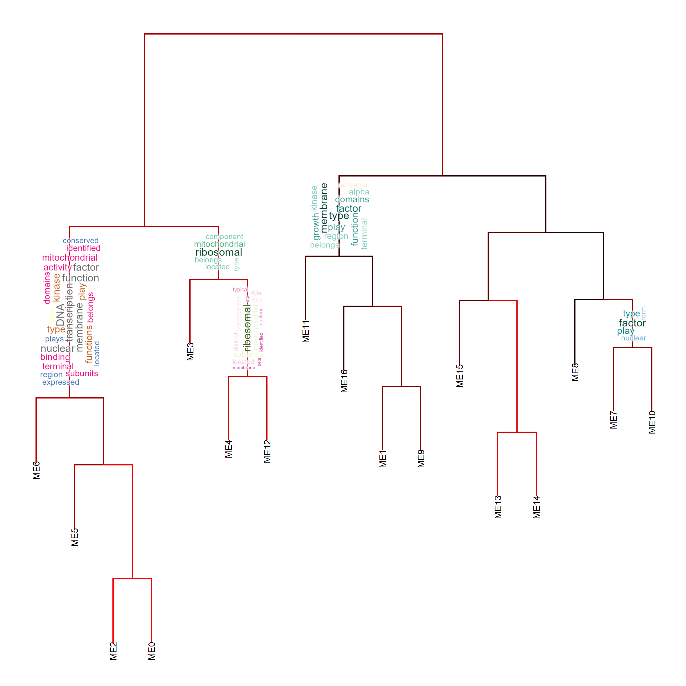
6 Annotating gene cluster dendrogram
6.1 Annotating by pyramid plots
The relationship between gene clusters are often investigated in clustering analysis like WGCNA. As workflows involving gene clustering analysis typically plot dendrogram and heatmap of module eigengenes using plotEigengeneNetworks, it is useful to combine with biotextgraph, which plot additional word information on a dendrogram with one line.
# WGCNA::plotEigengeneNetworks(mod$MEs, mod$colors, plotHeatmaps = FALSE)
plotEigengeneNetworksWithWords(MEs, modColors)
#> Bootstrap (r = 0.5)... Done.
#> Bootstrap (r = 0.6)... Done.
#> Bootstrap (r = 0.7)... Done.
#> Bootstrap (r = 0.8)... Done.
#> Bootstrap (r = 0.9)... Done.
#> Bootstrap (r = 1.0)... Done.
#> Bootstrap (r = 1.1)... Done.
#> Bootstrap (r = 1.2)... Done.
#> Bootstrap (r = 1.3)... Done.
#> Bootstrap (r = 1.4)... Done.
#> Input genes: 12
#>   Converted input genes: 7
#> Filter based on GeneSummary
#> Filtered 77 words (frequency and/or tfidf)
#> Input genes: 13
#>   Converted input genes: 13
#> Filter based on GeneSummary
#> Filtered 77 words (frequency and/or tfidf)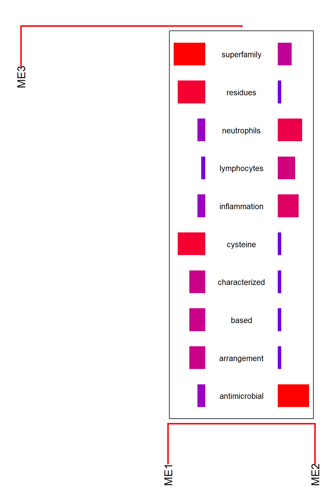
This calculates a dendrogram using pvclust internally in default. If you would like to plot segments involving only the specified gene cluster, use candidateNodes to specify the nodes.
plotEigengeneNetworksWithWords(MEs, modColors, candidateNodes=c("ME2"))
#> Bootstrap (r = 0.5)... Done.
#> Bootstrap (r = 0.6)... Done.
#> Bootstrap (r = 0.7)... Done.
#> Bootstrap (r = 0.8)... Done.
#> Bootstrap (r = 0.9)... Done.
#> Bootstrap (r = 1.0)... Done.
#> Bootstrap (r = 1.1)... Done.
#> Bootstrap (r = 1.2)... Done.
#> Bootstrap (r = 1.3)... Done.
#> Bootstrap (r = 1.4)... Done.
#> Input genes: 12
#>   Converted input genes: 7
#> Filter based on GeneSummary
#> Filtered 77 words (frequency and/or tfidf)
#> Input genes: 13
#>   Converted input genes: 13
#> Filter based on GeneSummary
#> Filtered 77 words (frequency and/or tfidf)
By default, the function calculates the frequency of common words across branches and plot the words that the differences between branches are large. By disabling takeIntersect, the function plots the frequent words for each branch.
plotEigengeneNetworksWithWords(MEs,
    modColors, takeIntersect=FALSE, candidateNodes=c("ME2"))
#> Bootstrap (r = 0.5)... Done.
#> Bootstrap (r = 0.6)... Done.
#> Bootstrap (r = 0.7)... Done.
#> Bootstrap (r = 0.8)... Done.
#> Bootstrap (r = 0.9)... Done.
#> Bootstrap (r = 1.0)... Done.
#> Bootstrap (r = 1.1)... Done.
#> Bootstrap (r = 1.2)... Done.
#> Bootstrap (r = 1.3)... Done.
#> Bootstrap (r = 1.4)... Done.
#> Input genes: 12
#>   Converted input genes: 7
#> Filter based on GeneSummary
#> Filtered 77 words (frequency and/or tfidf)
#> Input genes: 13
#>   Converted input genes: 13
#> Filter based on GeneSummary
#> Filtered 77 words (frequency and/or tfidf)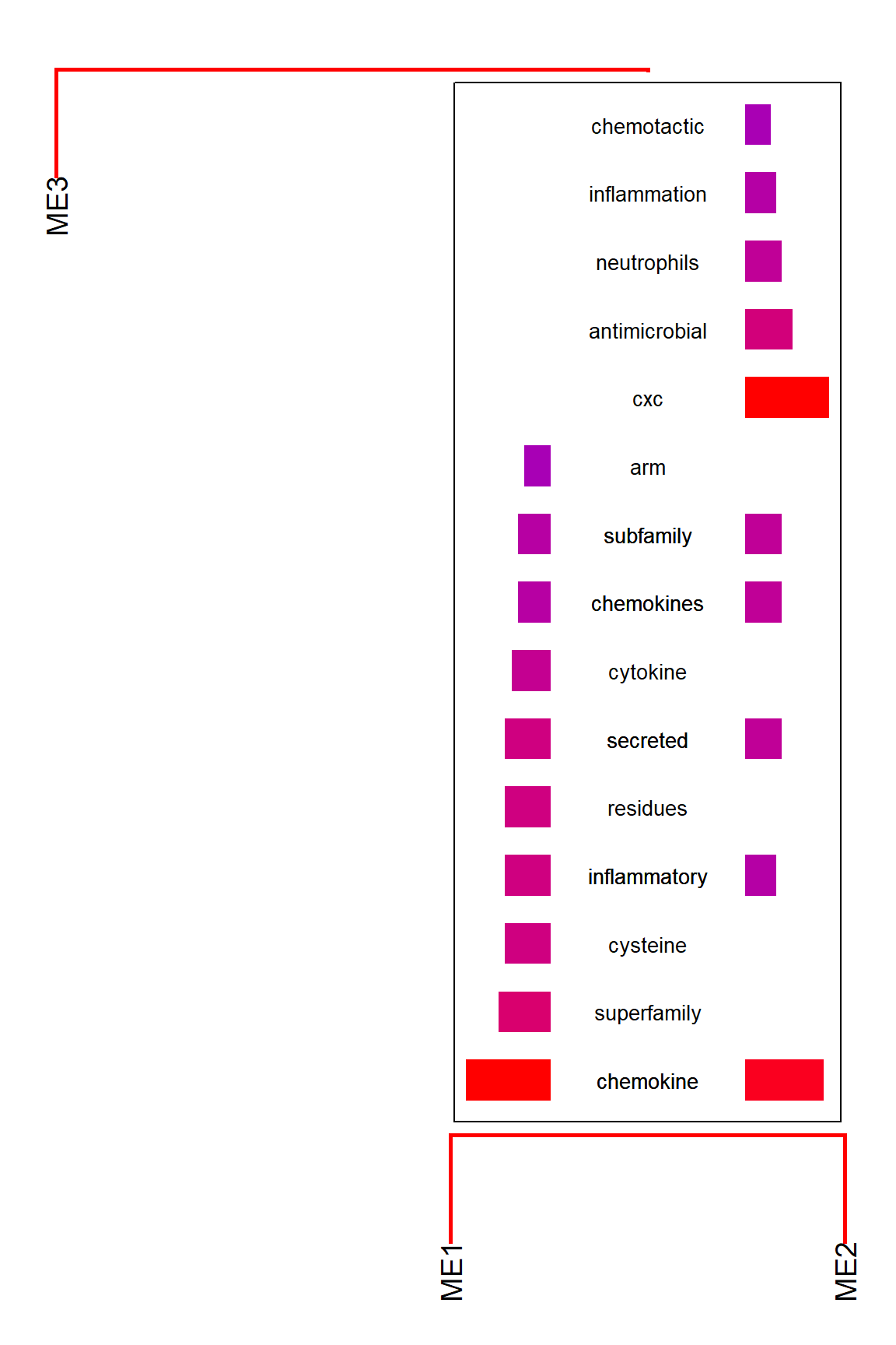
For examining enriched pathway names in the dendrograms, specify argList to refseq, like list(enrich="kegg").
plotEigengeneNetworksWithWords(MEs, modColors, type="words", argList=list(enrich="kegg"))
#> Bootstrap (r = 0.5)... Done.
#> Bootstrap (r = 0.6)... Done.
#> Bootstrap (r = 0.7)... Done.
#> Bootstrap (r = 0.8)... Done.
#> Bootstrap (r = 0.9)... Done.
#> Bootstrap (r = 1.0)... Done.
#> Bootstrap (r = 1.1)... Done.
#> Bootstrap (r = 1.2)... Done.
#> Bootstrap (r = 1.3)... Done.
#> Bootstrap (r = 1.4)... Done.
#> Input genes: 12
#>   Converted input genes: 7
#> Performing enrichment analysis
#> Filter based on GeneSummary
#> Filtered 77 words (frequency and/or tfidf)
#> Input genes: 13
#>   Converted input genes: 13
#> Performing enrichment analysis
#> Filter based on GeneSummary
#> Filtered 77 words (frequency and/or tfidf)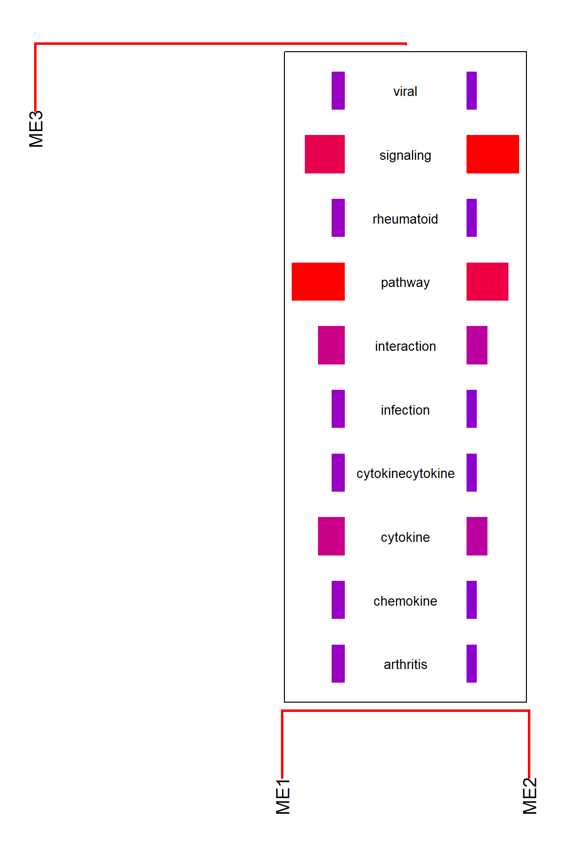
Other than textual information, we can simply annotate the dendrogram using enrichment analysis. Useful for inspecting how the branches of dendrogram contains pathway information.
plotEigengeneNetworksWithWords(MEs, modColors, type="enrich")
#> Bootstrap (r = 0.5)... Done.
#> Bootstrap (r = 0.6)... Done.
#> Bootstrap (r = 0.7)... Done.
#> Bootstrap (r = 0.8)... Done.
#> Bootstrap (r = 0.9)... Done.
#> Bootstrap (r = 1.0)... Done.
#> Bootstrap (r = 1.1)... Done.
#> Bootstrap (r = 1.2)... Done.
#> Bootstrap (r = 1.3)... Done.
#> Bootstrap (r = 1.4)... Done.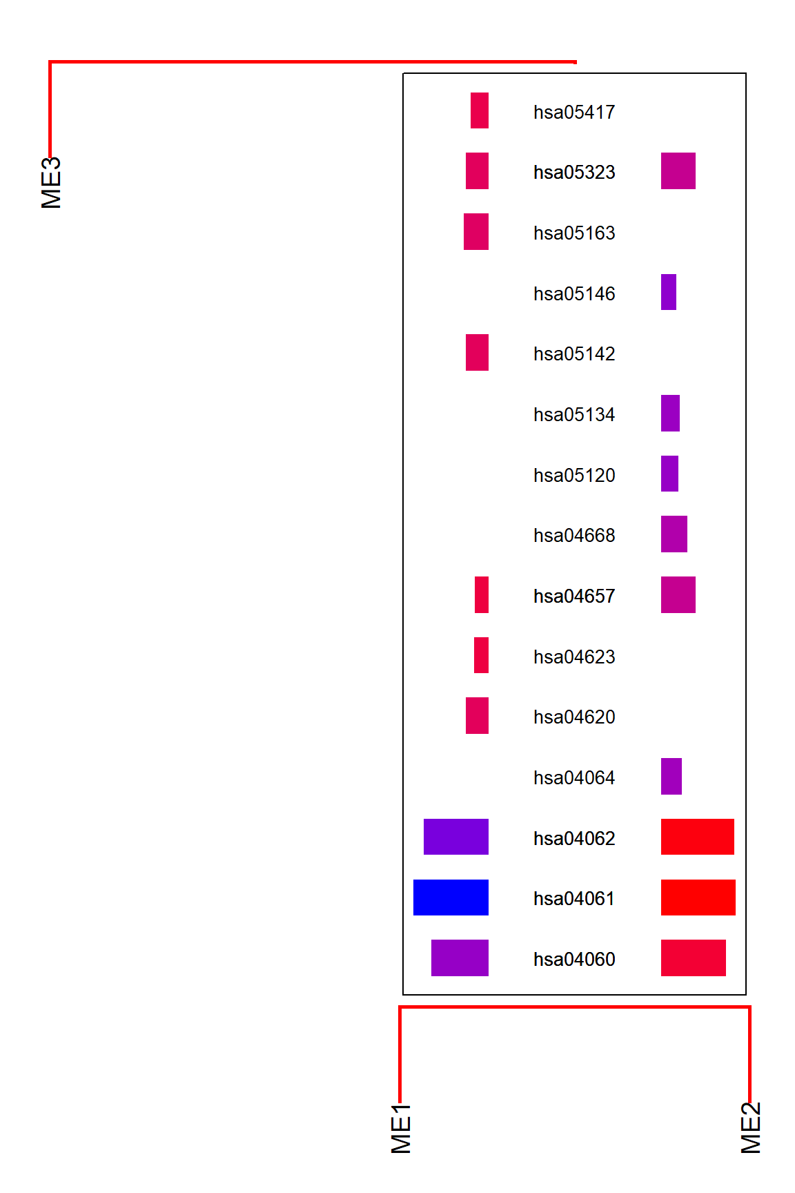
The column names for clusterProfiler results can be specified to showType.
plotEigengeneNetworksWithWords(MEs, modColors, type="enrich", showType="Description")
#> Bootstrap (r = 0.5)... Done.
#> Bootstrap (r = 0.6)... Done.
#> Bootstrap (r = 0.7)... Done.
#> Bootstrap (r = 0.8)... Done.
#> Bootstrap (r = 0.9)... Done.
#> Bootstrap (r = 1.0)... Done.
#> Bootstrap (r = 1.1)... Done.
#> Bootstrap (r = 1.2)... Done.
#> Bootstrap (r = 1.3)... Done.
#> Bootstrap (r = 1.4)... Done.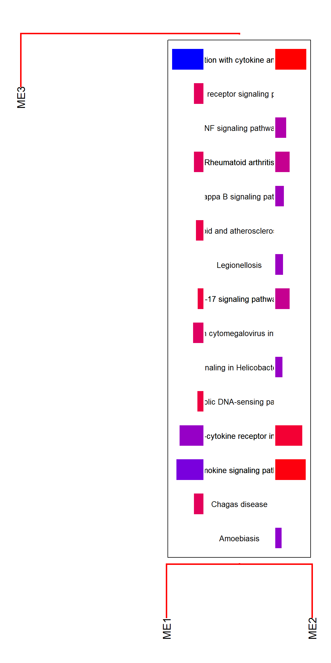
Text sizing and wrapping can be controlled by textSize and wrap.
plotEigengeneNetworksWithWords(MEs, modColors, type="enrich", showType="Description",
    textSize=1.5, wrap=30)
#> Bootstrap (r = 0.5)... Done.
#> Bootstrap (r = 0.6)... Done.
#> Bootstrap (r = 0.7)... Done.
#> Bootstrap (r = 0.8)... Done.
#> Bootstrap (r = 0.9)... Done.
#> Bootstrap (r = 1.0)... Done.
#> Bootstrap (r = 1.1)... Done.
#> Bootstrap (r = 1.2)... Done.
#> Bootstrap (r = 1.3)... Done.
#> Bootstrap (r = 1.4)... Done.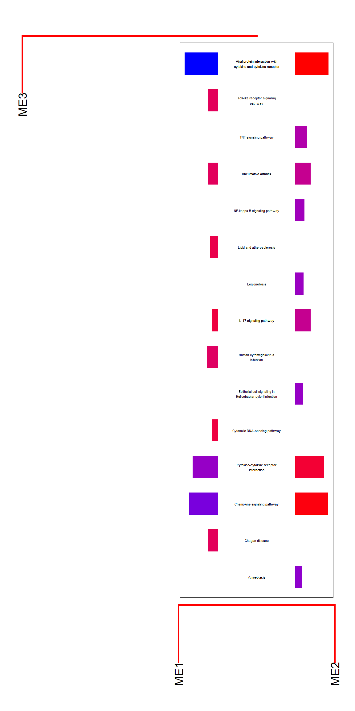
If you have a specifically interested pathway, use highlight to highlight the names in the dendrogram.
plotEigengeneNetworksWithWords(mod$MEs, mod$colors,
                               type="enrich", highlight=c("hsa04060"))+
  scale_y_continuous(expand=c(0,0.5))
#> Bootstrap (r = 0.5)... Done.
#> Bootstrap (r = 0.6)... Done.
#> Bootstrap (r = 0.7)... Done.
#> Bootstrap (r = 0.8)... Done.
#> Bootstrap (r = 0.9)... Done.
#> Bootstrap (r = 1.0)... Done.
#> Bootstrap (r = 1.1)... Done.
#> Bootstrap (r = 1.2)... Done.
#> Bootstrap (r = 1.3)... Done.
#> Bootstrap (r = 1.4)... Done.
#> 'select()' returned 1:1 mapping between keys and
#> columns
#> 'select()' returned 1:1 mapping between keys and
#> columns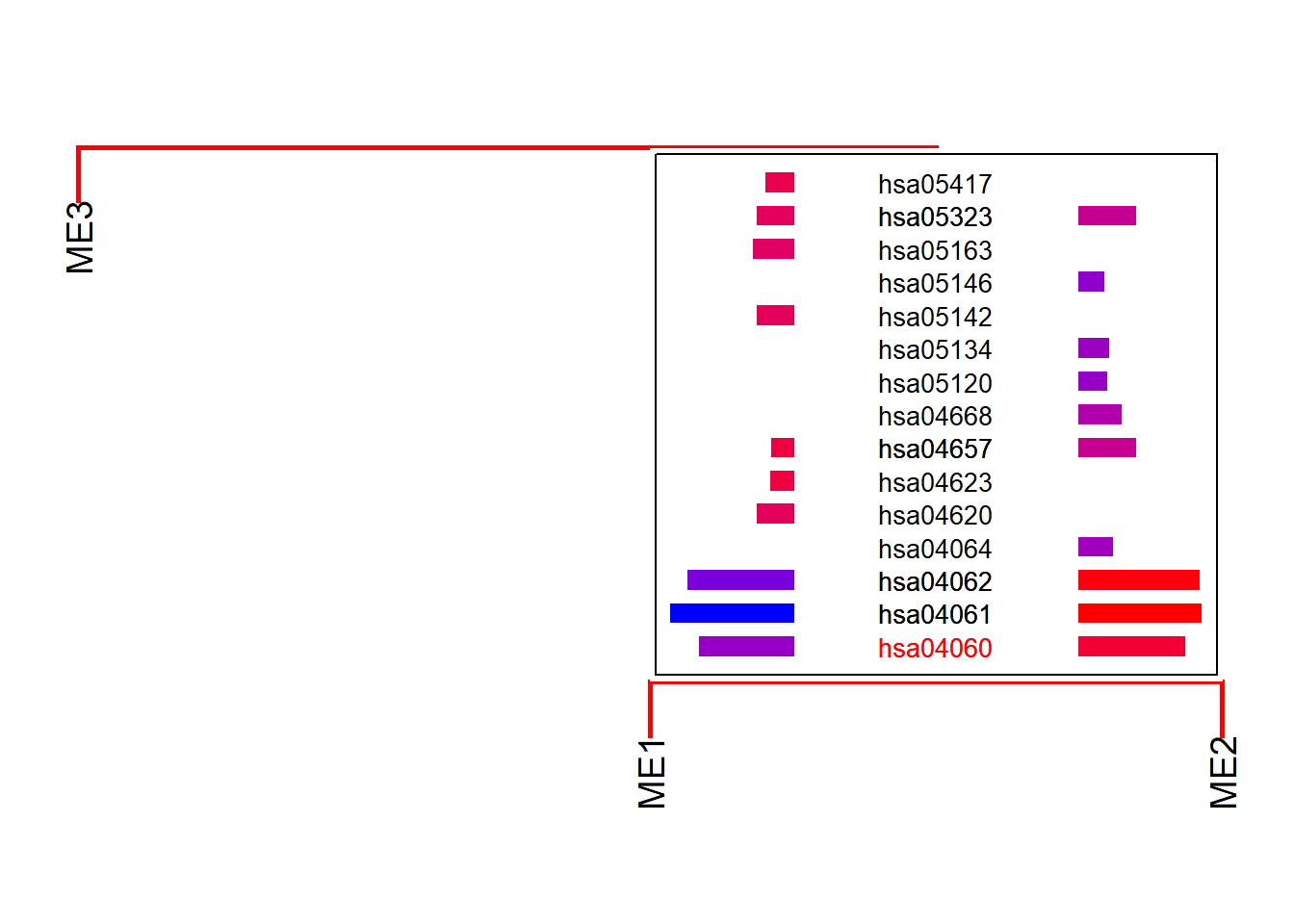
6.2 Annotating by word clouds
To plot the word cloud instead of pyramid plots, use useWC option. For scaling the word size, use wcScale option.
scale4 <- plotEigengeneNetworksWithWords(MEs, modColors, useWC=TRUE, candidateNodes=c("ME2"), wcScale=4)
#> Bootstrap (r = 0.5)... Done.
#> Bootstrap (r = 0.6)... Done.
#> Bootstrap (r = 0.7)... Done.
#> Bootstrap (r = 0.8)... Done.
#> Bootstrap (r = 0.9)... Done.
#> Bootstrap (r = 1.0)... Done.
#> Bootstrap (r = 1.1)... Done.
#> Bootstrap (r = 1.2)... Done.
#> Bootstrap (r = 1.3)... Done.
#> Bootstrap (r = 1.4)... Done.
#> Input genes: 25
#>   Converted input genes: 20
#> Filter based on GeneSummary
#> Filtered 77 words (frequency and/or tfidf)
#> Ignoring corThresh, automatically determine the value
#> threshold = 0.304
scale15 <- plotEigengeneNetworksWithWords(MEs, modColors, useWC=TRUE, candidateNodes=c("ME2"), wcScale=15)
#> Bootstrap (r = 0.5)... Done.
#> Bootstrap (r = 0.6)... Done.
#> Bootstrap (r = 0.7)... Done.
#> Bootstrap (r = 0.8)... Done.
#> Bootstrap (r = 0.9)... Done.
#> Bootstrap (r = 1.0)... Done.
#> Bootstrap (r = 1.1)... Done.
#> Bootstrap (r = 1.2)... Done.
#> Bootstrap (r = 1.3)... Done.
#> Bootstrap (r = 1.4)... Done.
#> Input genes: 25
#>   Converted input genes: 20
#> Filter based on GeneSummary
#> Filtered 77 words (frequency and/or tfidf)
#> Ignoring corThresh, automatically determine the value
#> threshold = 0.304
scale4 + scale15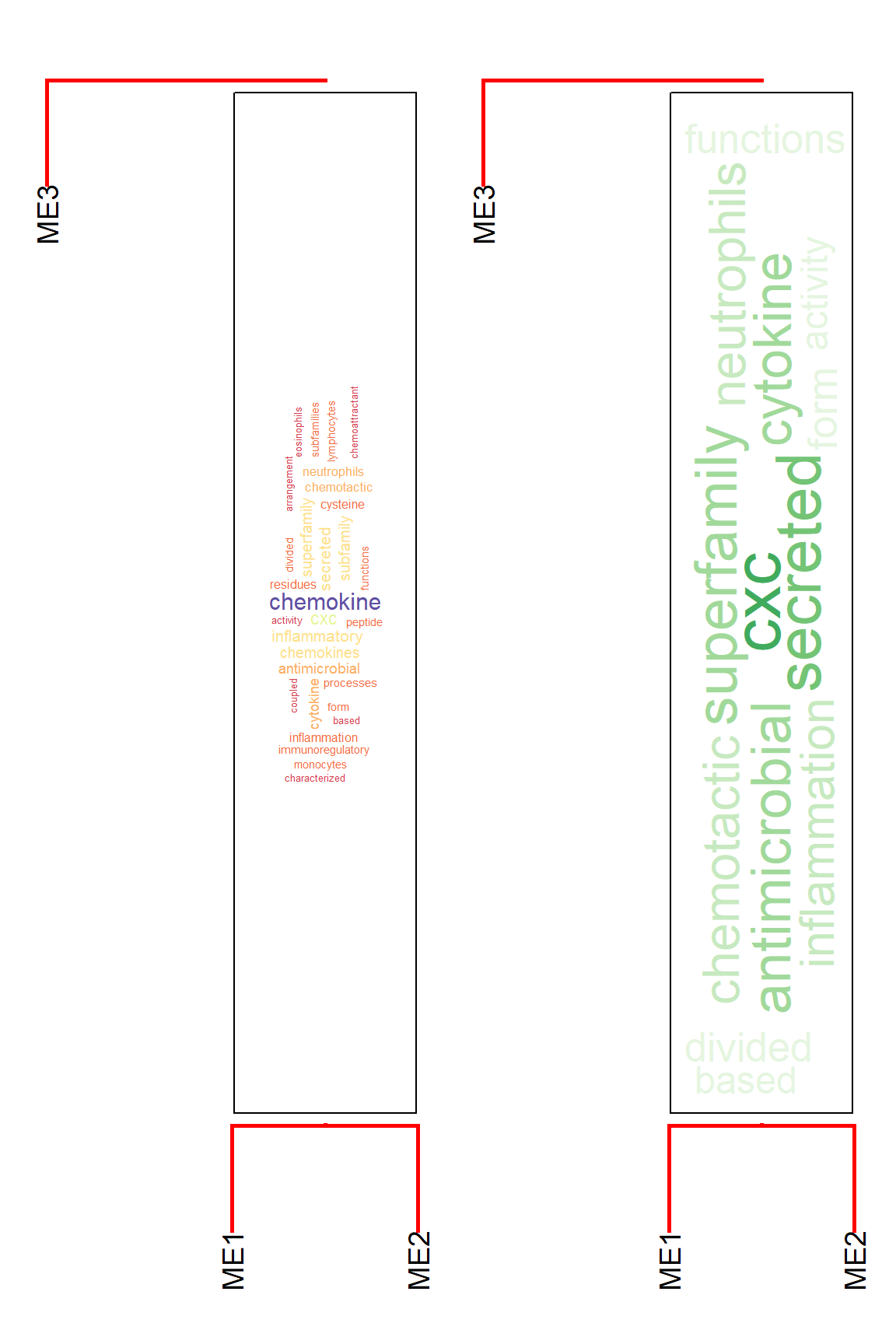
This uses ggwordcloud and a list specified by wcArgs is passed to the function.
plotEigengeneNetworksWithWords(MEs, modColors, useWC=TRUE, candidateNodes=c("ME2"), wcScale=15, wcArgs=list(rot.per=0))
#> Bootstrap (r = 0.5)... Done.
#> Bootstrap (r = 0.6)... Done.
#> Bootstrap (r = 0.7)... Done.
#> Bootstrap (r = 0.8)... Done.
#> Bootstrap (r = 0.9)... Done.
#> Bootstrap (r = 1.0)... Done.
#> Bootstrap (r = 1.1)... Done.
#> Bootstrap (r = 1.2)... Done.
#> Bootstrap (r = 1.3)... Done.
#> Bootstrap (r = 1.4)... Done.
#> Input genes: 25
#>   Converted input genes: 20
#> Filter based on GeneSummary
#> Filtered 77 words (frequency and/or tfidf)
#> Ignoring corThresh, automatically determine the value
#> threshold = 0.304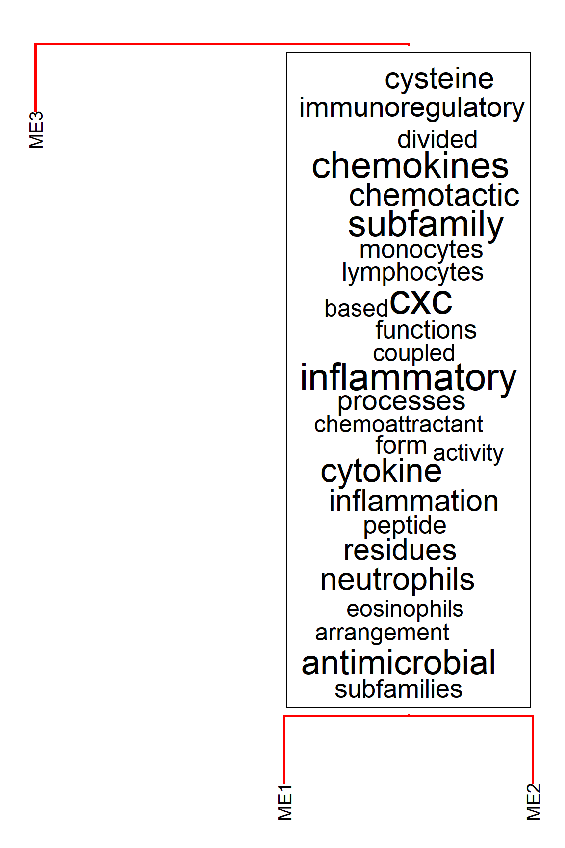
The horizontal plot can be specified by horiz=TRUE.
plotEigengeneNetworksWithWords(MEs,
                               modColors,
                               useWC=TRUE,
                               candidateNodes=c("ME2"),
                               wcScale=15,
                               wcArgs=list(rot.per=0),
                               horiz=TRUE)
#> Bootstrap (r = 0.5)... Done.
#> Bootstrap (r = 0.6)... Done.
#> Bootstrap (r = 0.7)... Done.
#> Bootstrap (r = 0.8)... Done.
#> Bootstrap (r = 0.9)... Done.
#> Bootstrap (r = 1.0)... Done.
#> Bootstrap (r = 1.1)... Done.
#> Bootstrap (r = 1.2)... Done.
#> Bootstrap (r = 1.3)... Done.
#> Bootstrap (r = 1.4)... Done.
#> Input genes: 25
#>   Converted input genes: 20
#> Filter based on GeneSummary
#> Filtered 77 words (frequency and/or tfidf)
#> Ignoring corThresh, automatically determine the value
#> threshold = 0.304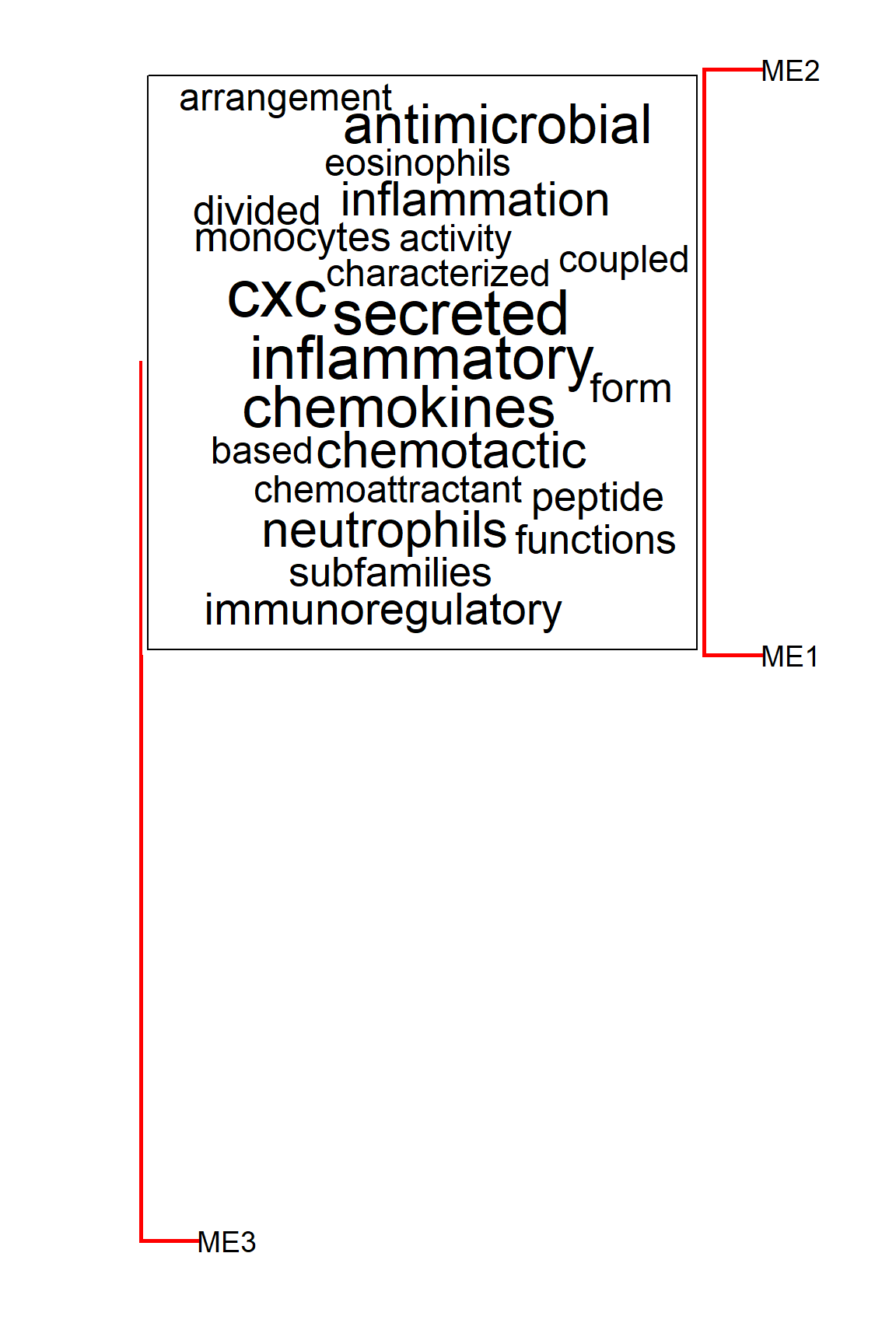
spacer can control the gaps above and below the grob on the dendrogram (y-axis).
horizontalSpacer can be used too for x-axis.
plotEigengeneNetworksWithWords(mod$MEs, mod$colors,
                               type="enrich", highlight=c("hsa04060"), spacer=0.2)+
    scale_y_continuous(expand=c(0,0.5))
#> Bootstrap (r = 0.5)... Done.
#> Bootstrap (r = 0.6)... Done.
#> Bootstrap (r = 0.7)... Done.
#> Bootstrap (r = 0.8)... Done.
#> Bootstrap (r = 0.9)... Done.
#> Bootstrap (r = 1.0)... Done.
#> Bootstrap (r = 1.1)... Done.
#> Bootstrap (r = 1.2)... Done.
#> Bootstrap (r = 1.3)... Done.
#> Bootstrap (r = 1.4)... Done.
#> 'select()' returned 1:1 mapping between keys and
#> columns
#> 'select()' returned 1:1 mapping between keys and
#> columns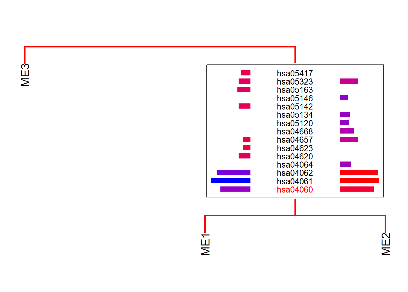
plotEigengeneNetworksWithWords(mod$MEs, mod$colors, useWC=TRUE,
                               spacer=0.2, horizontalSpacer=0.1)+
    scale_y_continuous(expand=c(0,0.5))
#> Bootstrap (r = 0.5)... Done.
#> Bootstrap (r = 0.6)... Done.
#> Bootstrap (r = 0.7)... Done.
#> Bootstrap (r = 0.8)... Done.
#> Bootstrap (r = 0.9)... Done.
#> Bootstrap (r = 1.0)... Done.
#> Bootstrap (r = 1.1)... Done.
#> Bootstrap (r = 1.2)... Done.
#> Bootstrap (r = 1.3)... Done.
#> Bootstrap (r = 1.4)... Done.
#> Input genes: 25
#> 'select()' returned 1:1 mapping between keys and
#> columns
#>   Converted input genes: 20
#> Filter based on GeneSummary
#> Filtered 77 words (frequency and/or tfidf)
#> Ignoring corThresh, automatically determine the value
#> threshold = 0.304
#> Scale for size is already present.
#> Adding another scale for size, which will replace the
#> existing scale.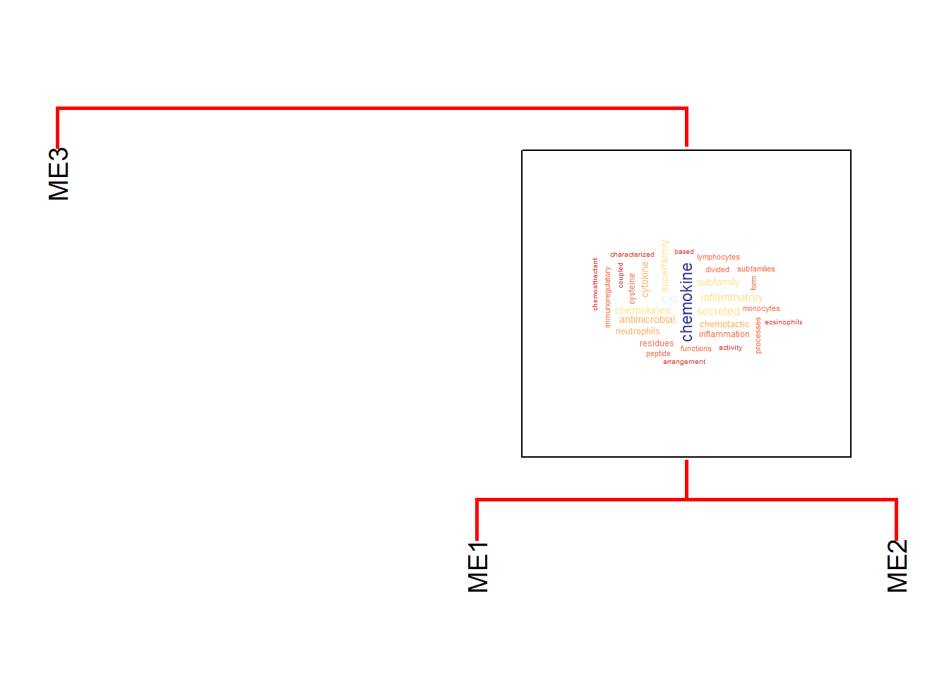
By specifying returnGlobOnly, the grobs with the position in the dendrogram can be returned.
gro <- plotEigengeneNetworksWithWords(mod$MEs, mod$colors, candidateNodes=c("ME2"),
                               returnGlobOnly=TRUE)
#> Bootstrap (r = 0.5)... Done.
#> Bootstrap (r = 0.6)... Done.
#> Bootstrap (r = 0.7)... Done.
#> Bootstrap (r = 0.8)... Done.
#> Bootstrap (r = 0.9)... Done.
#> Bootstrap (r = 1.0)... Done.
#> Bootstrap (r = 1.1)... Done.
#> Bootstrap (r = 1.2)... Done.
#> Bootstrap (r = 1.3)... Done.
#> Bootstrap (r = 1.4)... Done.
#> Input genes: 12
#> 'select()' returned 1:1 mapping between keys and
#> columns
#>   Converted input genes: 7
#> Filter based on GeneSummary
#> Filtered 77 words (frequency and/or tfidf)
#> Input genes: 13
#> 'select()' returned 1:1 mapping between keys and
#> columns
#>   Converted input genes: 13
#> Filter based on GeneSummary
#> Filtered 77 words (frequency and/or tfidf)
ggplotify::as.ggplot(gro[[1]]$plot)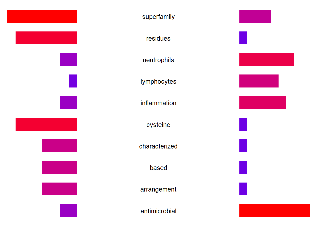
6.3 Decorating wordclouds
If needed, wordclouds can be filtered by ggfx or using shadowtext. In this case, border is set to FALSE and the background will be transparent for resulting grobs. If shadowtext is needed, specify bg.colour argument. If ggfx is needed, specify the filter function in useggfx and parameters in ggfxParams.
library(ggfx)
plotEigengeneNetworksWithWords(MEs, modColors, useWC=TRUE, candidateNodes=c("ME2"), wcScale=4,
    bg.colour="grey80")+ scale_y_continuous(expand=c(0,3))
#> Bootstrap (r = 0.5)... Done.
#> Bootstrap (r = 0.6)... Done.
#> Bootstrap (r = 0.7)... Done.
#> Bootstrap (r = 0.8)... Done.
#> Bootstrap (r = 0.9)... Done.
#> Bootstrap (r = 1.0)... Done.
#> Bootstrap (r = 1.1)... Done.
#> Bootstrap (r = 1.2)... Done.
#> Bootstrap (r = 1.3)... Done.
#> Bootstrap (r = 1.4)... Done.
#> Input genes: 25
#> 'select()' returned 1:1 mapping between keys and
#> columns
#>   Converted input genes: 20
#> Filter based on GeneSummary
#> Filtered 77 words (frequency and/or tfidf)
#> Ignoring corThresh, automatically determine the value
#> threshold = 0.304
#> Warning in brewer.pal(10, sample(row.names(RColorBrewer::brewer.pal.info), : n too large, allowed maximum for palette Pastel1 is 9
#> Returning the palette you asked for with that many colors
#> Scale for size is already present.
#> Adding another scale for size, which will replace the
#> existing scale.
#> border is set to FALSE as bg.colour is not NULL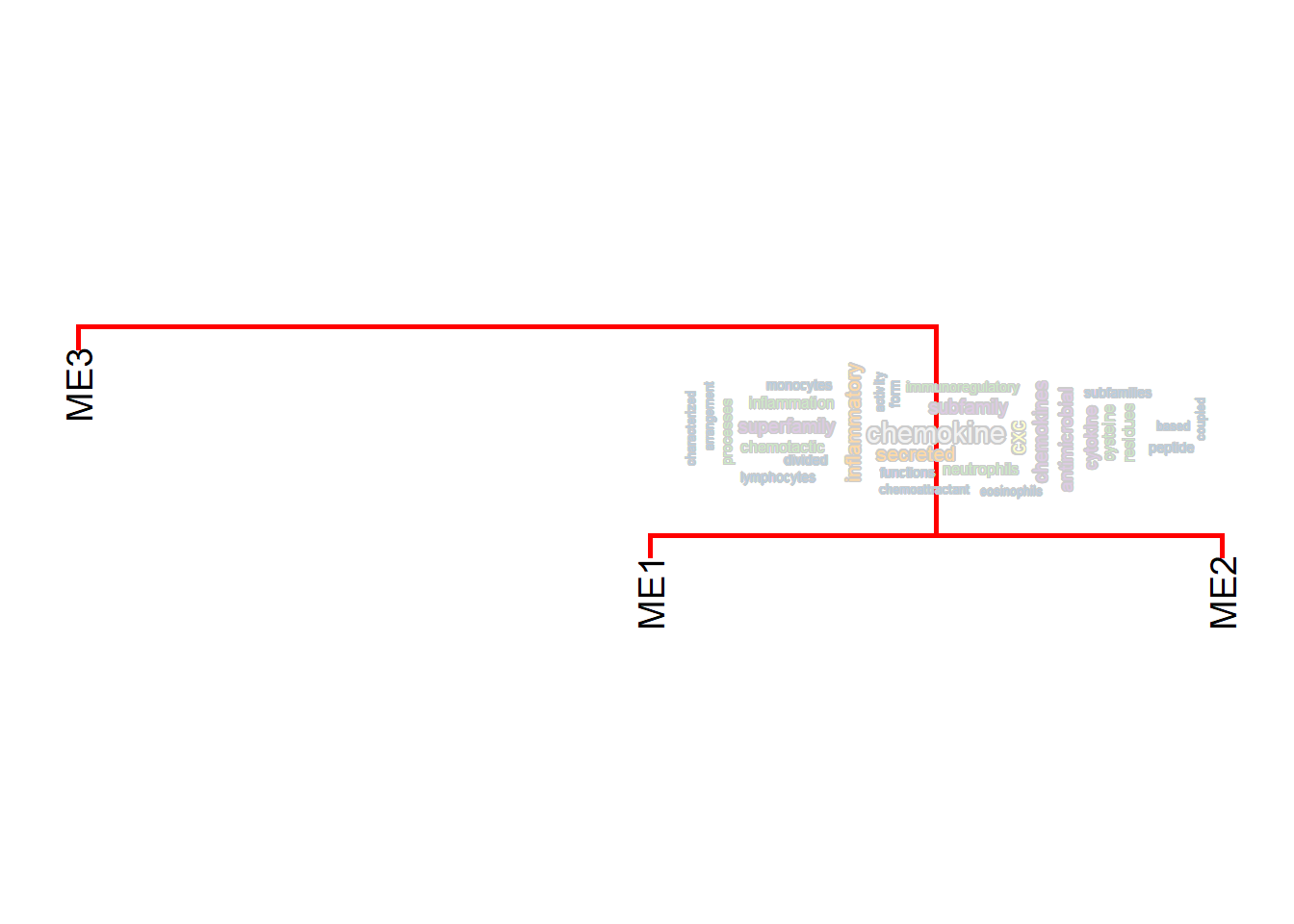
plotEigengeneNetworksWithWords(MEs, modColors, useWC=TRUE, candidateNodes=c("ME2"), wcScale=4,
    useggfx="with_outer_glow", ggfxParams=list(colour="white",expand=5))+ scale_y_continuous(expand=c(0,3))
#> Bootstrap (r = 0.5)... Done.
#> Bootstrap (r = 0.6)... Done.
#> Bootstrap (r = 0.7)... Done.
#> Bootstrap (r = 0.8)... Done.
#> Bootstrap (r = 0.9)... Done.
#> Bootstrap (r = 1.0)... Done.
#> Bootstrap (r = 1.1)... Done.
#> Bootstrap (r = 1.2)... Done.
#> Bootstrap (r = 1.3)... Done.
#> Bootstrap (r = 1.4)... Done.
#> Input genes: 25
#> 'select()' returned 1:1 mapping between keys and
#> columns
#>   Converted input genes: 20
#> Filter based on GeneSummary
#> Filtered 77 words (frequency and/or tfidf)
#> Ignoring corThresh, automatically determine the value
#> threshold = 0.304
#> Warning in brewer.pal(10, sample(row.names(RColorBrewer::brewer.pal.info), : n too large, allowed maximum for palette Blues is 9
#> Returning the palette you asked for with that many colors
#> Scale for size is already present.
#> Adding another scale for size, which will replace the
#> existing scale.
#> border is set to FALSE as useggfx is not NULL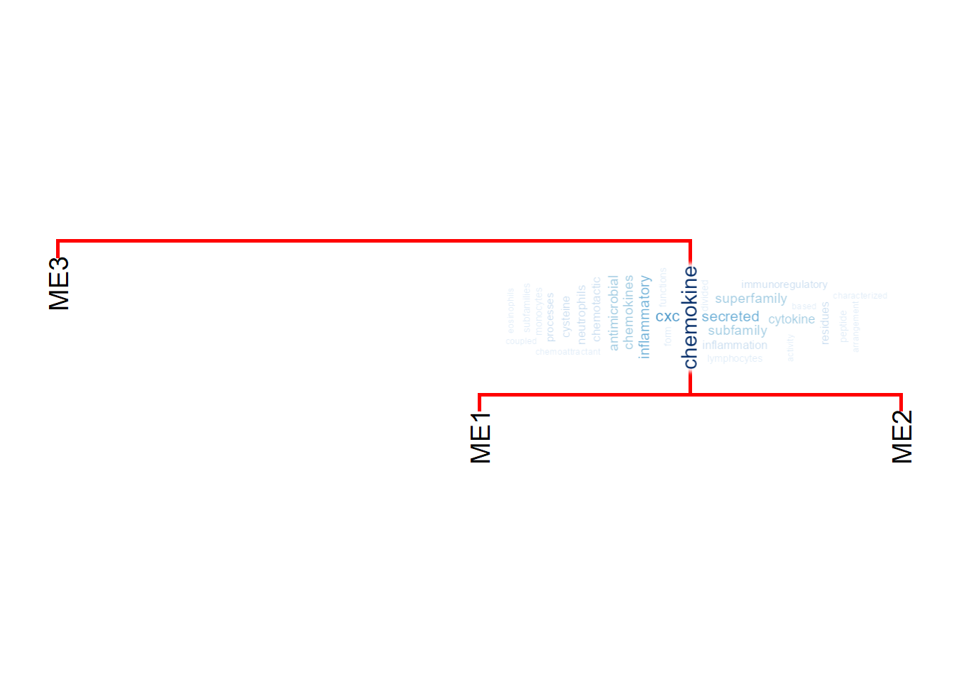
The below example shows using the other dendrogram like those produced by WGCNA combining the parameters.
library(ggfx)
load("./blockwiseModule.rda")
MEs <- bwmod$MEs
modColors <- bwmod$colors
plotEigengeneNetworksWithWords(MEs,useWC=TRUE,
                              modColors, candidateNodes=c("ME11","ME3","ME7","ME6","ME12"),
                              useggfx="with_outer_glow", useRandomColor=TRUE,
                              ggfxParams=list(colour="white",expand=3),
                              wcScale=6, wcArgs=list(shape="square",
                              min.freq=1, max.words=Inf, rot.per=0.5,random.order=FALSE))
#> Bootstrap (r = 0.49)... Done.
#> Bootstrap (r = 0.6)... Done.
#> Bootstrap (r = 0.69)... Done.
#> Bootstrap (r = 0.8)... Done.
#> Bootstrap (r = 0.89)... Done.
#> Bootstrap (r = 1.0)... Done.
#> Bootstrap (r = 1.09)... Done.
#> Bootstrap (r = 1.2)... Done.
#> Bootstrap (r = 1.29)... Done.
#> Bootstrap (r = 1.4)... Done.
#> Input genes: 5822
#>   Converted input genes: 4793
#> Filter based on GeneSummary
#> Filtered 77 words (frequency and/or tfidf)
#> Ignoring corThresh, automatically determine the value
#> threshold = 0
#> Input genes: 15534
#>   Converted input genes: 12187
#> Filter based on GeneSummary
#> Filtered 77 words (frequency and/or tfidf)
#> Ignoring corThresh, automatically determine the value
#> threshold = 0
#> Input genes: 1926
#>   Converted input genes: 1558
#> Filter based on GeneSummary
#> Filtered 77 words (frequency and/or tfidf)
#> Ignoring corThresh, automatically determine the value
#> threshold = 0
#> Input genes: 860
#>   Converted input genes: 673
#> Filter based on GeneSummary
#> Filtered 77 words (frequency and/or tfidf)
#> Ignoring corThresh, automatically determine the value
#> threshold = 0.102
#> Input genes: 275
#>   Converted input genes: 260
#> Filter based on GeneSummary
#> Filtered 77 words (frequency and/or tfidf)
#> Ignoring corThresh, automatically determine the value
#> threshold = 0.001
#> border is set to FALSE as useggfx is not NULL