5 Visualization
stana offers visualization functions that can interpret the profiled data.
library(stana)
library(ComplexHeatmap)
5.1 plotSNVSummary and plotSNVInfo
These functions can be used to plot the information related to SNV, which can be used to inspect the overview of profiled SNVs.
load("../hd_meta.rda")
stana <- loadMIDAS2("../merge_uhgg", cl=hd_meta, candSp="102478")
#>   102478
#>   s__Clostridium_A leptum
#>     Number of snps: 77431
#>     Number of samples: 31
#>   102478
#>   s__Clostridium_A leptum
#>     Number of genes: 150996
#>     Number of samples: 32
plotSNVSummary(stana, "102478")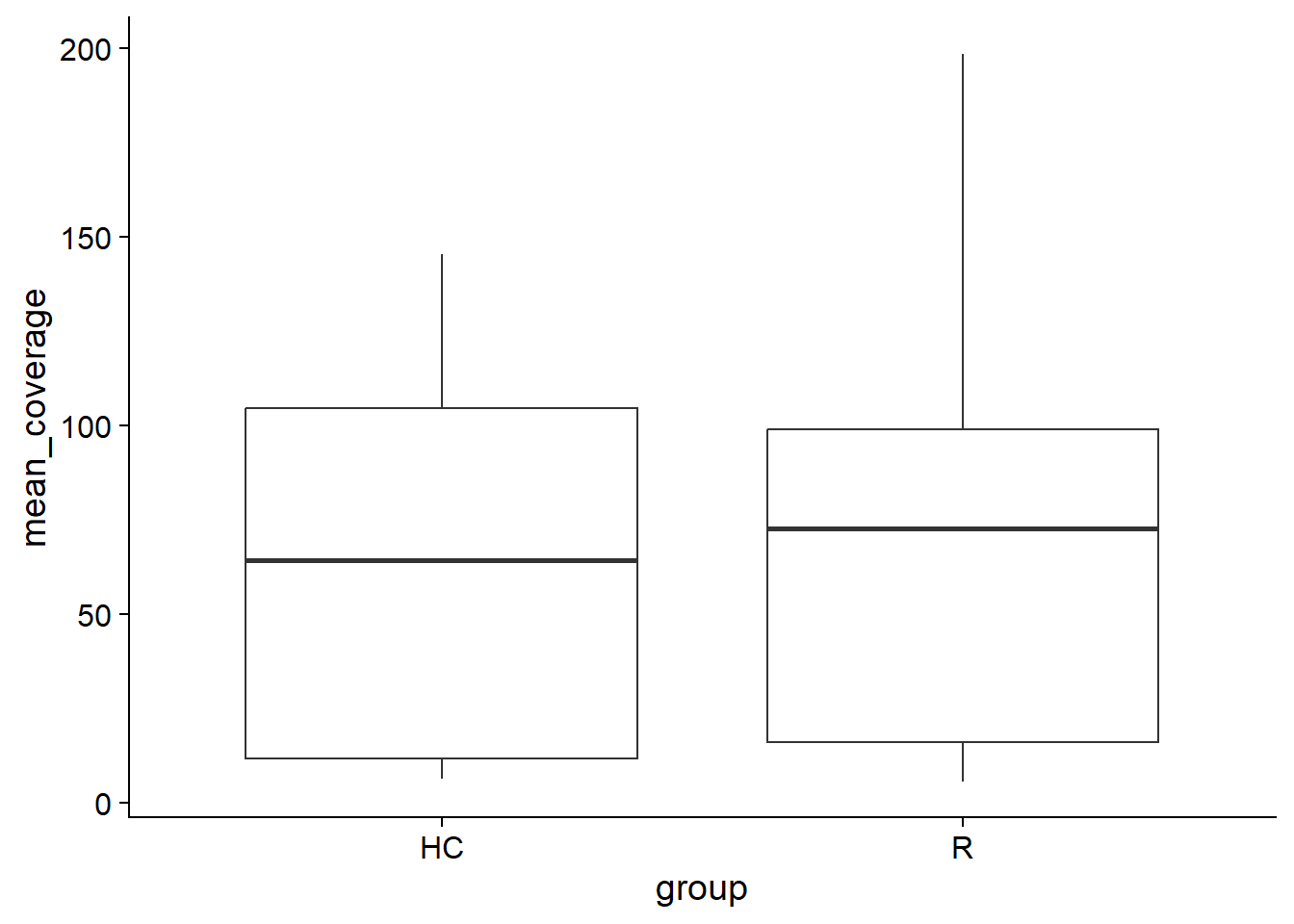
plotSNVInfo(stana, "102478")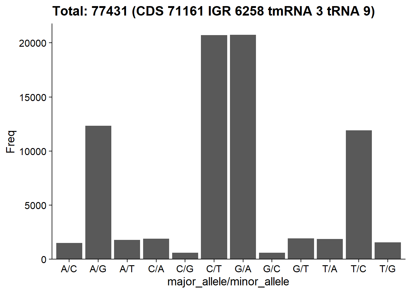
5.3 plotMAFHist
This functions plots the histogram of MAF for the candidate species.
plotMAFHist(stana, "102478")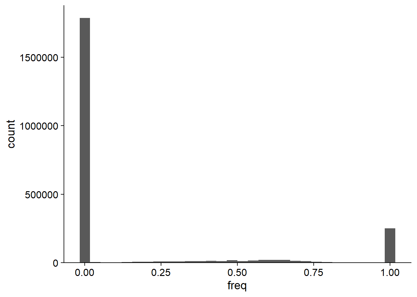
5.4 plotCoverage
This function plots the coverage of the canddiate species across the group.
plotCoverage(stana, "102478")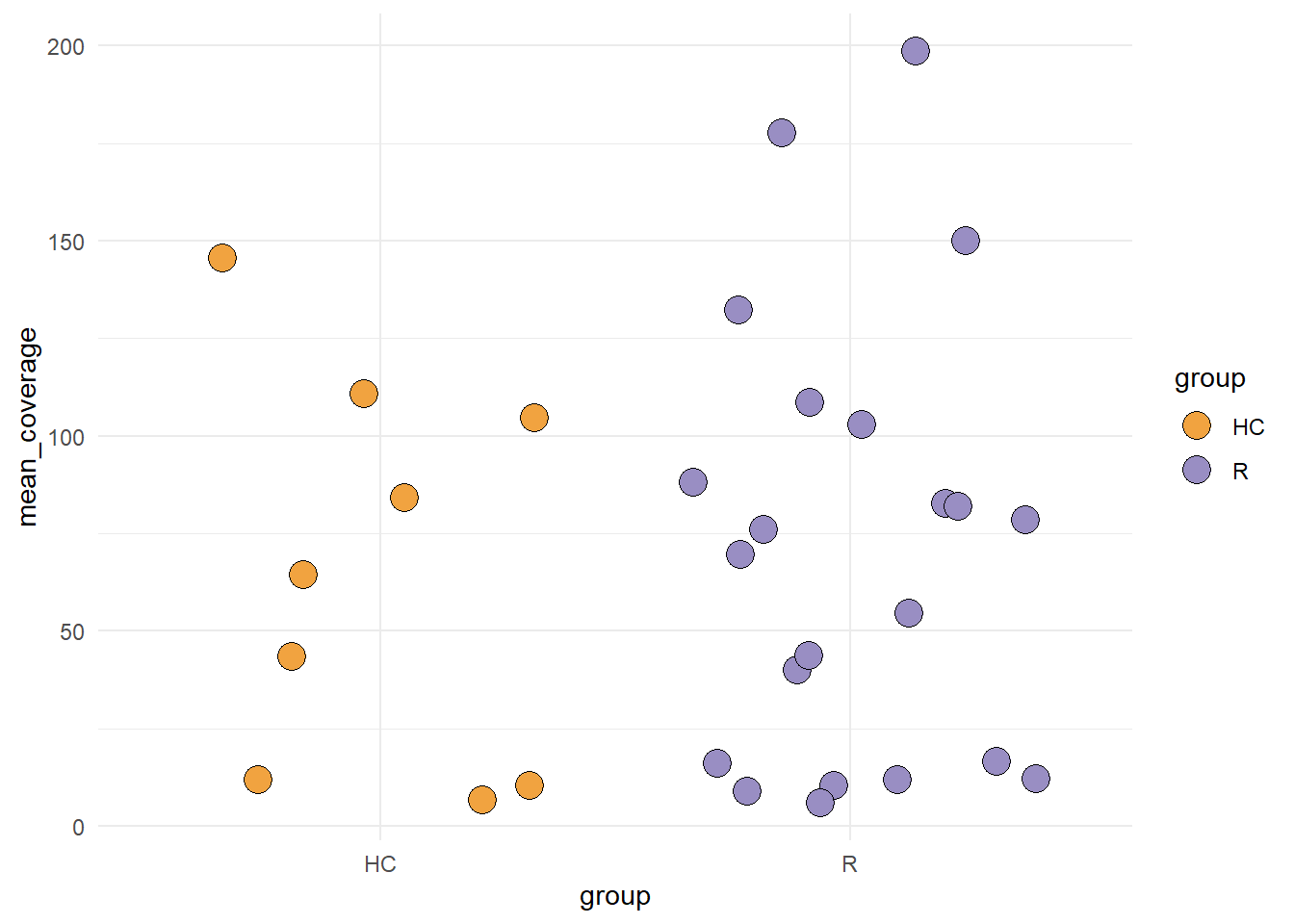
5.5 plotPCA
You can plot principal component analysis results using prcomp by plotPCA function across grouping specified. If no group is specified, No_Group label is assigned to all the samples.
mt <- loadmetaSNV("../metasnv_sample_out/",just_species = TRUE)
mt <- loadmetaSNV("../metasnv_sample_out/", candSp=mt[1])
#>   Loading refGenome1clus
plotPCA(mt, species=getID(mt)[1])
#> After filtering: 1022 SNVs
#> $refGenome1clus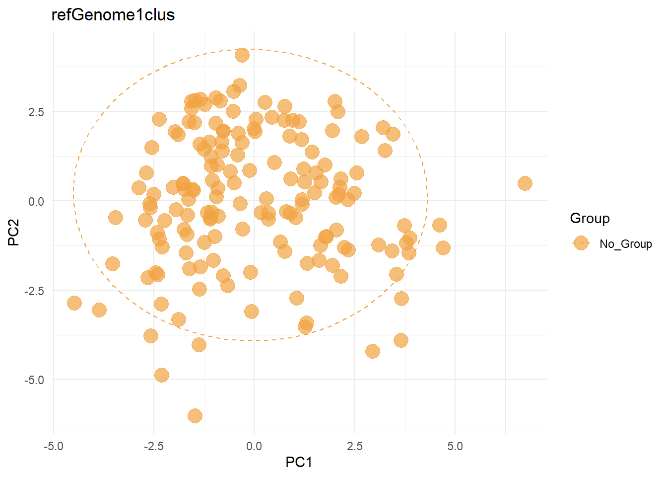
5.6 plotDist
Plot the heatmap of distance matrix with grouping variables using pheatmap.
library(pheatmap)
plotDist(stana, "102478", target="snps")
#> # Performing dist in 102478 target is snps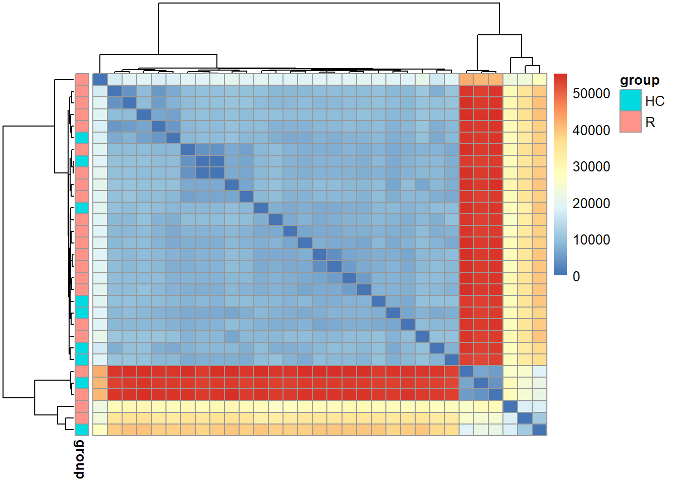
Plot using the subset of the SNV.
stana <- siteFilter(stana, "102478", site_type=="4D")
#> # total of 27533 obtained from 77431
plotDist(stana, "102478", target="snps")
#> # Performing dist in 102478 target is snps
#> # The set SNV ID information (27533) is used.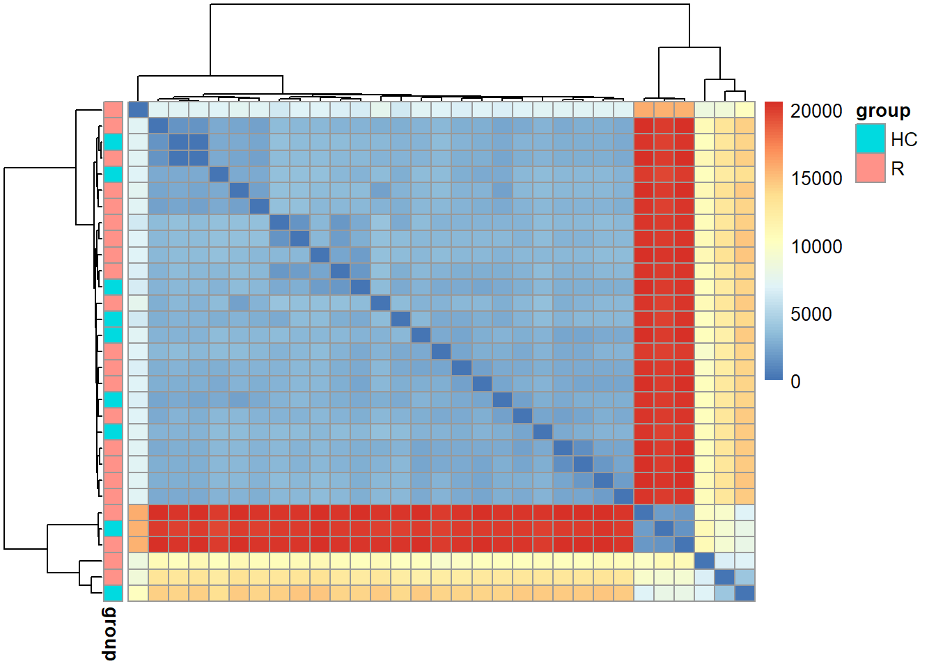
5.7 plotCirclize
This function can be used to circlize plot, which can link the information related to MAF or SNV with gene copy number analysis. The function needs the snpsInfo slot filled with the data having genome_id, gene_id and position column. For MIDAS2 and inStrain, the packge automatically infers the genome_id.
library(circlize)
plotCirclize(stana, "102478", genomeId="UHGG143505", thresh_snp_gene = 150)
#> Type is MIDAS2
#> Features not provided, default to sample_counts
#> Genome ID in SNV information:
#>   UHGG143505_1: 179 - 5439351, number of position: 77431
#> Genome ID: UHGG143505
#> Included position: 987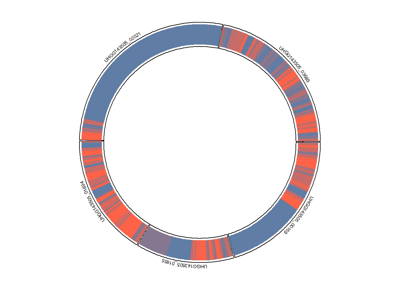
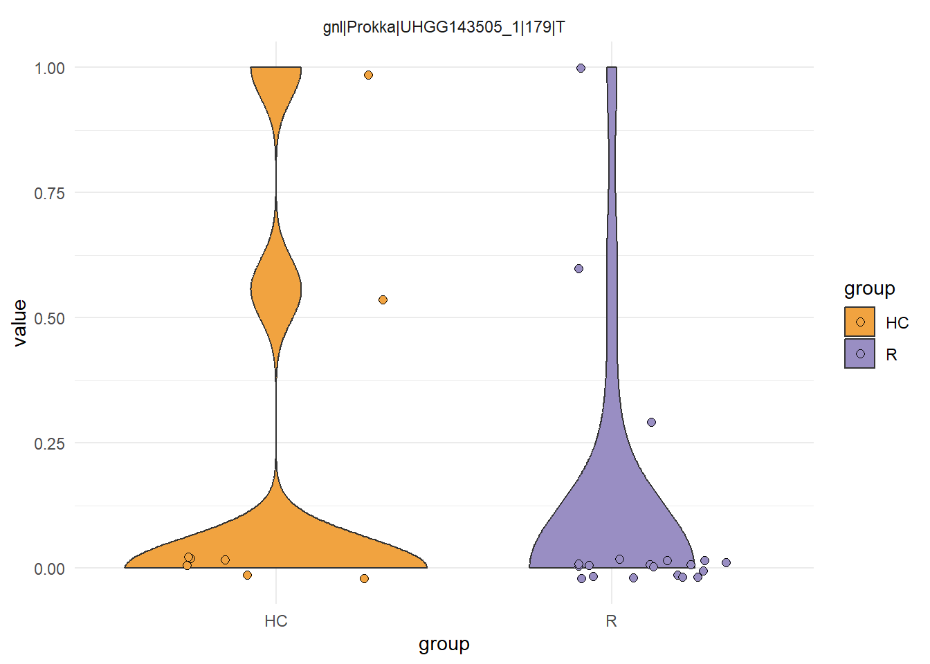
5.8 Visualization of gene copy numbers
The violin plot of gene copy numbers can be plotted by plotGenes.
load("../hd_meta.rda")
stana <- loadMIDAS2("../merge_uhgg", cl=hd_meta, candSp="102478")
#>   102478
#>   s__Clostridium_A leptum
#>     Number of snps: 77431
#>     Number of samples: 31
#>   102478
#>   s__Clostridium_A leptum
#>     Number of genes: 150996
#>     Number of samples: 32
plotGenes(stana, "102478", c("UHGG000186_00531","UHGG000186_00521"))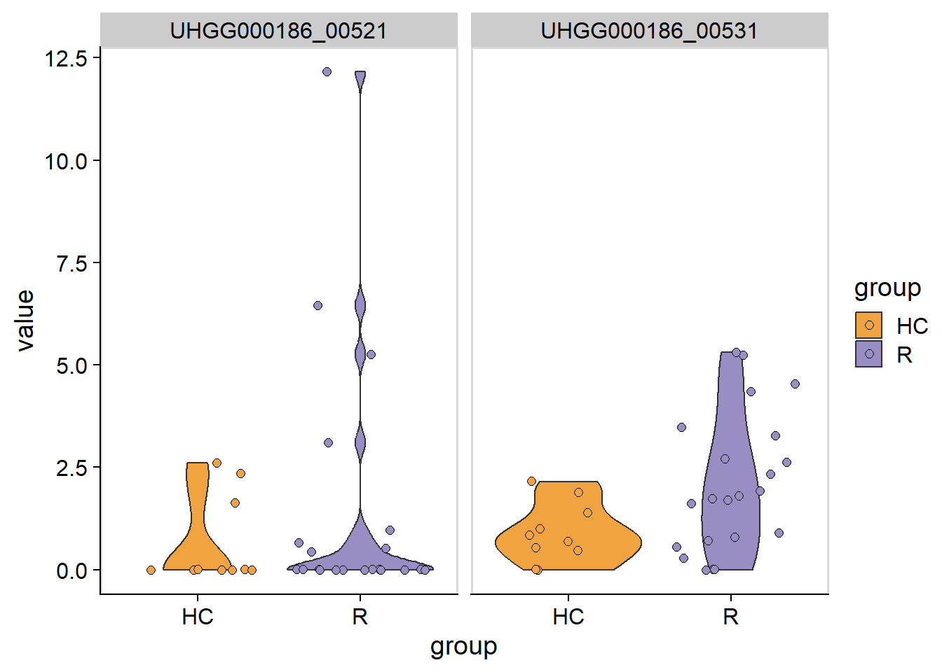
Default color mapping can be changed by changeColors.
stana <- changeColors(stana, c("blue","red"))
plotGenes(stana, "102478", c("UHGG000186_00531","UHGG000186_00521"))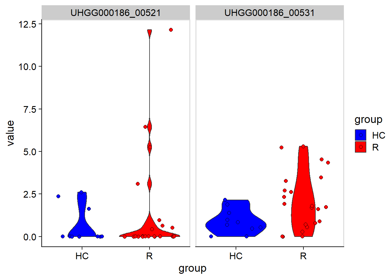
5.9 Visualization of phylogenetic tree
See 3.1 for the functions like inferAndPlotTree for visualizing the phylogenetic tree inferred by various methods.
5.10 Visualization of functional analysis results
See 4 for the functions like plotHeatmap and plotKEGGPathway.
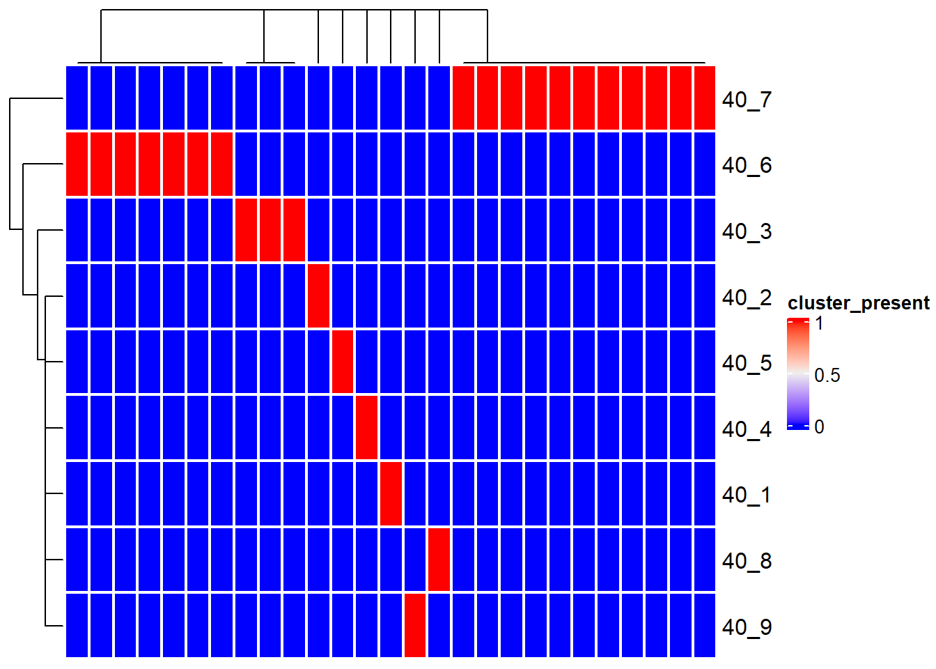
5.11 Visualization of inStrain results
For the specific software, the imported inStrain compare profiles can be visualized. The loaded genome-wide comparison table and strain cluster table can be visualized using genomeHeatmap and strainClusterHeatmap by ComplexHeatmap. For genomeHeatmap, typically population ANI or consensus ANI are plotted, but all the columns listed in genomeWide_compare.tsv can be plotted. The parameters to be passed to Heatmap can be specified with heatmapArgs. If cluster information (getCl(stana)) is available or cl is specified, the columns will be split to present the grouping. Please refer to the documentation of inStrain for popANI and conANI.
instr_chk <- "GUT_GENOME142015"
instr <- loadInStrain("../inStrain_out", instr_chk)
genomeHeatmap(instr, instr_chk, column = "popANI", heatmapArgs = list(show_column_name=FALSE))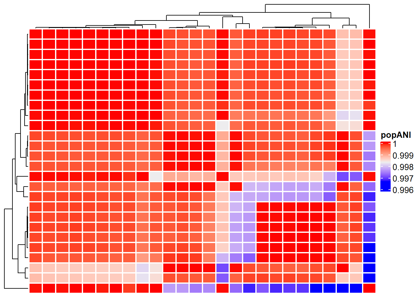
strainClusterHeatmap(instr, instr_chk, heatmapArgs = list(show_column_name=FALSE))