3 Statistial analysis

stana provides functions to perform statistical analysis on the metagenotyping results based on loaded data.

library(stana)
library(phangorn)
library(ggtree)
library(ggstar)
## Examine sample object
load(system.file("extdata", "sysdata.rda", package = "stana"))

3.1 Consensus sequence calling

The consensus sequence calling can be performed using SNV MAF matrix (or the matrix converted from the allelic counts). It can filter the confident and user-defined positions and output the multiple sequence alignment in fastaList slot. The MIDAS and MIDAS2 output provides various statistics of SNVs that can be used for the filtering. The implementation is similar to that in MIDAS. Here we use pair-wise distances of sequences calculated by dist.ml in the default amino acid model (JC69), and performs neighbor-joining tree estimation by NJ.

## The consensusSeq* is prepared, but consensusSeq function can automatically 
## choose which functions to use
stana <- consensusSeqMIDAS2(stana, species="100003", verbose=FALSE)
#> # Beginning calling for 100003
#> # Original Site number: 5019
#> #  Profiled samples: 11
#> #  Included samples: 11

## Tree estimation and visualization by `phangorn` and `ggtree`
dm <- dist.ml(getSlot(stana, "fastaList")[["100003"]])
tre <- NJ(dm)
tre <- groupOTU(tre, getSlot(stana, "cl"))
tp <- ggtree(tre, aes(color=.data$group),
             layout='circular') +
        geom_tippoint(size=3) +
        ggtree::scale_color_manual(values=getSlot(stana, "colors"))
tp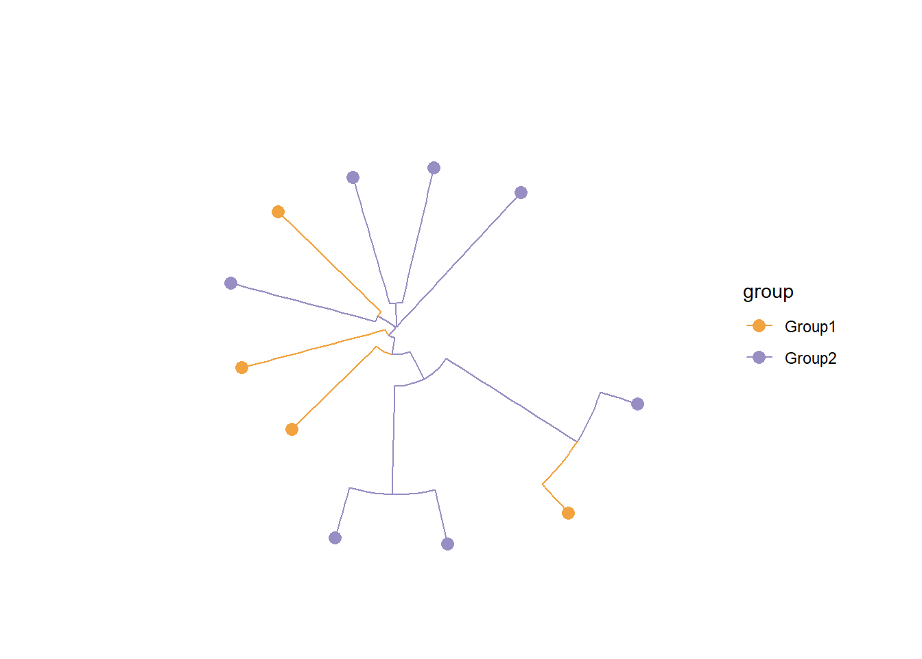

The sequences are stored as phyDat class object in fastaList slot, the list with the species ID as name.

stana <- stana |>
    consensusSeq(argList=list(site_prev=0.8))
#> # Beginning calling for 100003
#> # Original Site number: 5019
#> #  Profiled samples: 11
#> #  Included samples: 11
getFasta(stana)[[1]]
#> 11 sequences with 4214 character and 2782 different site patterns.
#> The states are a c g t

Matrix of characters can be returned by return_mat=TRUE. This does not return stana object.

mat <- stana |>
    consensusSeq(argList=list(site_prev=0.8, return_mat=TRUE))
#> # Beginning calling for 100003
#> # Original Site number: 5019
#> #  Profiled samples: 11
#> #  Included samples: 11
mat |> dim()
#> [1]   11 4214

You can use the MSA stored in fastaList slot to infer the phylogenetic tree of your choices. The inferAndPlotTree function can be used to internally infer and plot the tree based on grouping. dist_method is set to dist.ml by default, and you can pass arguments to the function by tree_args.

library(phangorn)
stana <- inferAndPlotTree(stana, dist_method="dist.hamming", tree_args=list(exclude="all"))
getTree(stana)[[1]]
#> 
#> Phylogenetic tree with 11 tips and 10 internal nodes.
#> 
#> Tip labels:
#>   ERR1711593, ERR1711594, ERR1711596, ERR1711598, ERR1711603, ERR1711605, ...
#> 
#> Rooted; includes branch lengths.

Owning to the powerful functions in ggtree and ggtreeExtra, you can visualize the tree based on the metadata. You should set data.frame containing covariates to stana object by setMetadata function. And specify the covariates to meta argument in plotTree.

## Make example metadata
samples <- getSlot(stana, "snps")[["100003"]] |> colnames()
metadata <- data.frame(
    row.names=samples,
    treatment=factor(sample(1:3, length(samples), replace=TRUE)),
    marker=runif(length(samples))
)

## Set metadata
stana <- setMetadata(stana, metadata)

## Call consensus sequence
## Infer and plot tree based on metadata
stana <- stana |>
  consensusSeq(argList=list(site_prev=0.95)) |>
  inferAndPlotTree(meta=c("treatment","marker"))
#> # Beginning calling for 100003
#> # Original Site number: 5019
#> #  Profiled samples: 11
#> #  Included samples: 11
getFasta(stana)[[1]]
#> 11 sequences with 896 character and 625 different site patterns.
#> The states are a c g t
getTree(stana)[[1]]
#> 
#> Phylogenetic tree with 11 tips and 10 internal nodes.
#> 
#> Tip labels:
#>   ERR1711593, ERR1711594, ERR1711596, ERR1711598, ERR1711603, ERR1711605, ...
#> 
#> Rooted; includes branch lengths.
getSlot(stana, "treePlotList")[[1]]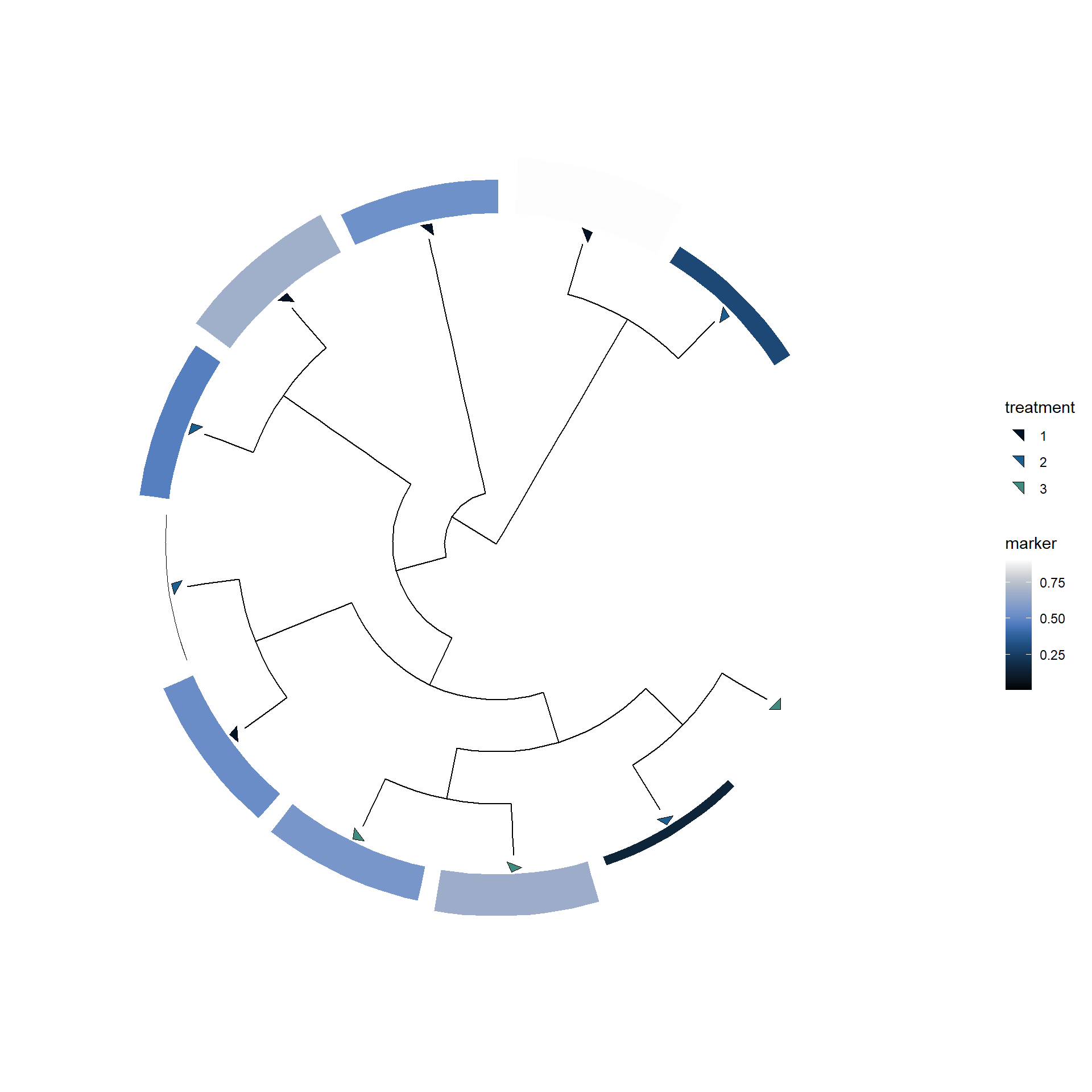

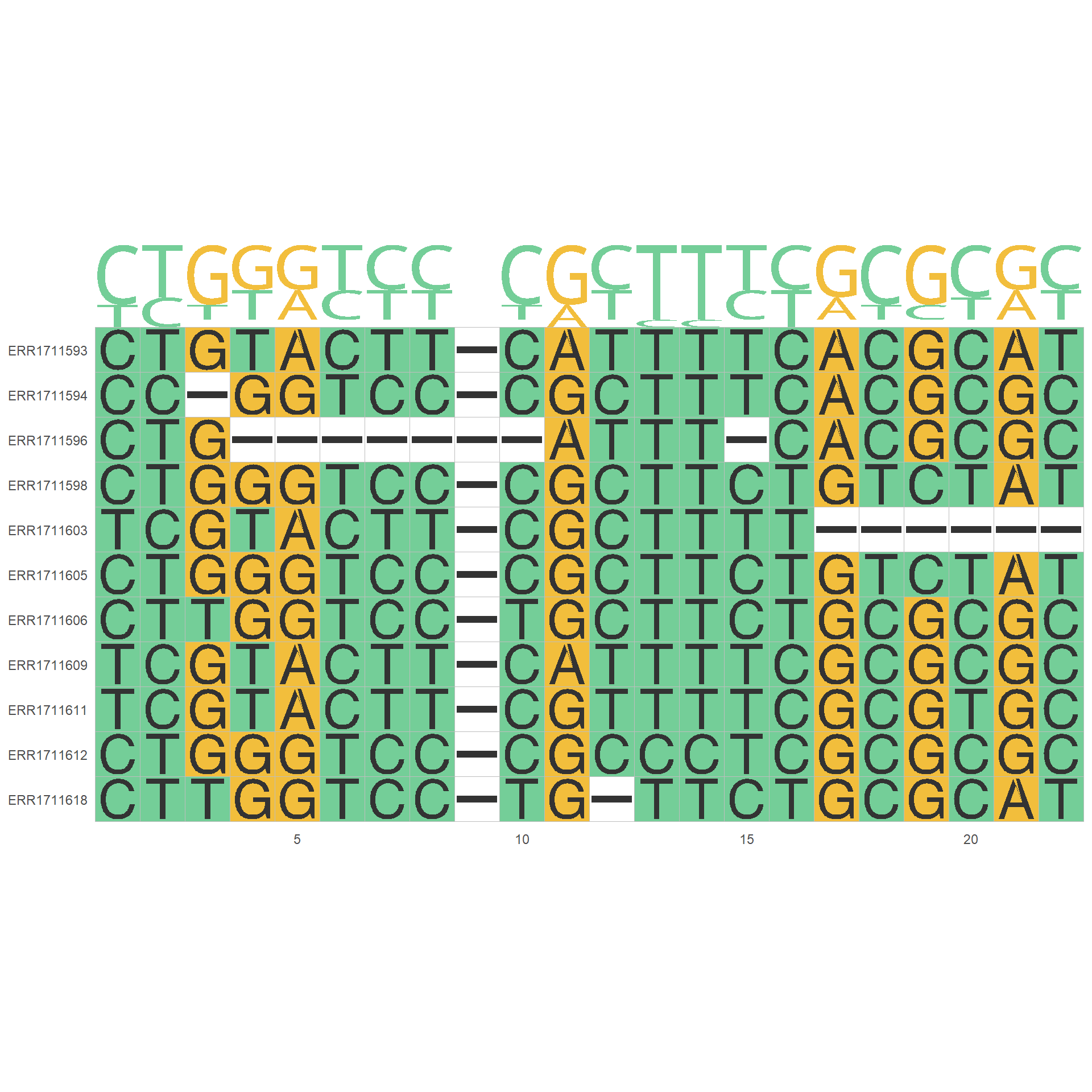
The site_list is supported for the usecase such as calling limited to the certain gene regions. The below example calls the MSA in specific gene ID and output plot by ggmsa.

## get snpsInfo slot and filter to variants in specific gene IDs
cand_ids <- stana::getSlot(stana, "snpsInfo")[["100003"]] %>%
    dplyr::filter(gene_id=="UHGG000008_01913") %>%
    row.names()

## Call sequence
stana <- consensusSeqMIDAS2(stana, "100003", site_list=cand_ids)
#> # Beginning calling for 100003
#> # Original Site number: 5019
#> #  Profiled samples: 11
#> #  Included samples: 11
#> # site_list specified: 22

## Plot
if (requireNamespace("ggmsa")) {
    library(ggmsa)
    phangorn::write.phyDat(getFasta(stana)[["100003"]],
                           "test.fasta", format="fasta")
    ggmsa::ggmsa("test.fasta",seq_name = TRUE)+ ggmsa::geom_seqlogo()
}

3.2 Nonnegative matrix factorization

The loaded or calculated matrix can be used for the nonnegative matrix factorization (NMF) for the unsupervised identifications of factors within species. This calculates factor x sample and sample to feature matrix, and possibly finds the pattern for the within-species diversity. The results can be summarized by the functions such as plotAbundanceWithinSpecies.

The input can be SNV, gene, or gene family (KO) copy number table. The matrix can contain NA or -1 (zero depth at the position), so filtering should be performed. The NMF::nmf function or NNLM::nnmf function can be used for this purpose. By default, estimate is set to FALSE but if set to TRUE, it performs the estimation of rank within estimate_range. This assumes that multiple subspecies are in the samples and is not applicable where only one subspecies should be present. It chooses the rank based on the cophenetic correlation coefficient when the function uses the R package NMF, but the package implements a variety of algorithms and the rank selection method. Also, if NNLM, the rank selection based on cross-validation by randomly assigning the NA in the cell in the matrix, is performed.

The function outputs the related statistics like the proportion of NA or zero value, the relative profiles of factors after the estimation, or the features presented in each factor.

The method is set to snmf/r by default in NMF. For the larger matrix, the NNML function can be used for the faster computation by setting nnlm_flag to TRUE.

library(NMF)
stana <- NMF(stana, "100003", estimate=TRUE)[[1]]
#> # NMF started 100003, target: kos, method: snmf/r
#> # Original features: 20
#> # Original samples: 16
#> # Original matrix NA: NA
#> # Original matrix zero: 0.781
#> # Selecting KL loss
#> # Filtered features: 20
#> # Filtered samples: 16
#> # Chosen rank:3
#> # Rank 3
#> Mean relative abundances: 0.4506259 0.3696346 0.1797395 
#> Present feature per factor: 18 14 13
getSlot(stana, "nmf")
#> NULL

The users can specify the rank. The NMF slot stores the list of NMF results (or NNLM results) per species.

stana <- NMF(stana, "100003", rank=3, beta=0.001)
#> # NMF started 100003, target: kos, method: snmf/r
#> # Original features: 20
#> # Original samples: 16
#> # Original matrix NA: NA
#> # Original matrix zero: 0.781
#> # Selecting KL loss
#> # Filtered features: 20
#> # Filtered samples: 16
#> # Rank 3
#> Mean relative abundances: 0.4391153 0.3652978 0.1955869 
#> Present feature per factor: 15 11 12
getSlot(stana, "NMF")
#> $`100003`
#> <Object of class: NMFfit>
#>  # Model:
#>   <Object of class:NMFstd>
#>   features: 20 
#>   basis/rank: 3 
#>   samples: 16 
#>  # Details:
#>   algorithm:  snmf/r 
#>   seed:  random 
#>   RNG: 10403L, 624L, ..., -1119848976L [a0b56536ecb759f07f21b4b252fb5db8]
#>   distance metric:  <function> 
#>   residuals:  5.628987 
#>   parameters: beta=0.001 
#>   Iterations: 65 
#>   Timing:
#>      user  system elapsed 
#>      0.05    0.00    0.05

The resulting stana object can be used with the other function. plotAbundanceWithinSpecies plots the (relative) sample profiles per sample using the grouping criteria in stana object.

plotAbundanceWithinSpecies(stana, "100003", tss=TRUE)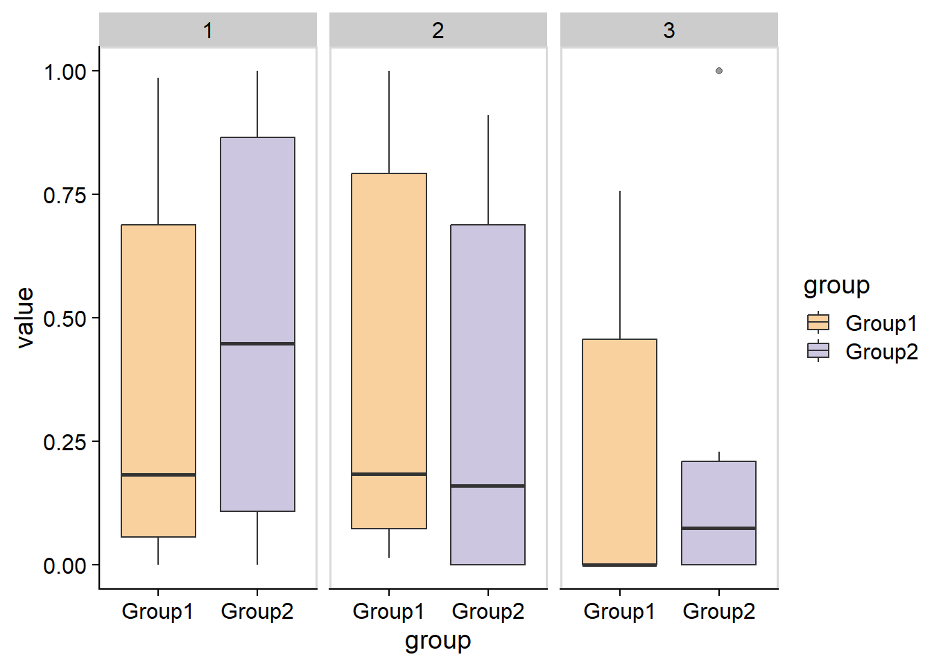

The data can be obtained using return_data.

plotAbundanceWithinSpecies(stana, "100003", tss=TRUE, return_data=TRUE) %>% head()
#>                     1          2         3  group
#> ERR1711593 0.98582990 0.01417010 0.0000000 Group1
#> ERR1711594 0.85247014 0.14752986 0.0000000 Group1
#> ERR1711596 0.19498362 0.04848823 0.7565282 Group1
#> ERR1711598 0.17024848 0.22117519 0.6085763 Group1
#> ERR1711599 0.00000000 1.00000000 0.0000000 Group1
#> ERR1711602 0.01749079 0.98250921 0.0000000 Group1

The basis corresponds to the factor to feature matrix. This can represent functional profiles if the KO or gene copy number tables are used for the NMF. This information can be summarized to matrix of KEGG PATHWAY information using pathwayWithFactor.

library(pheatmap)
pheatmap(pathwayWithFactor(stana, "100003"))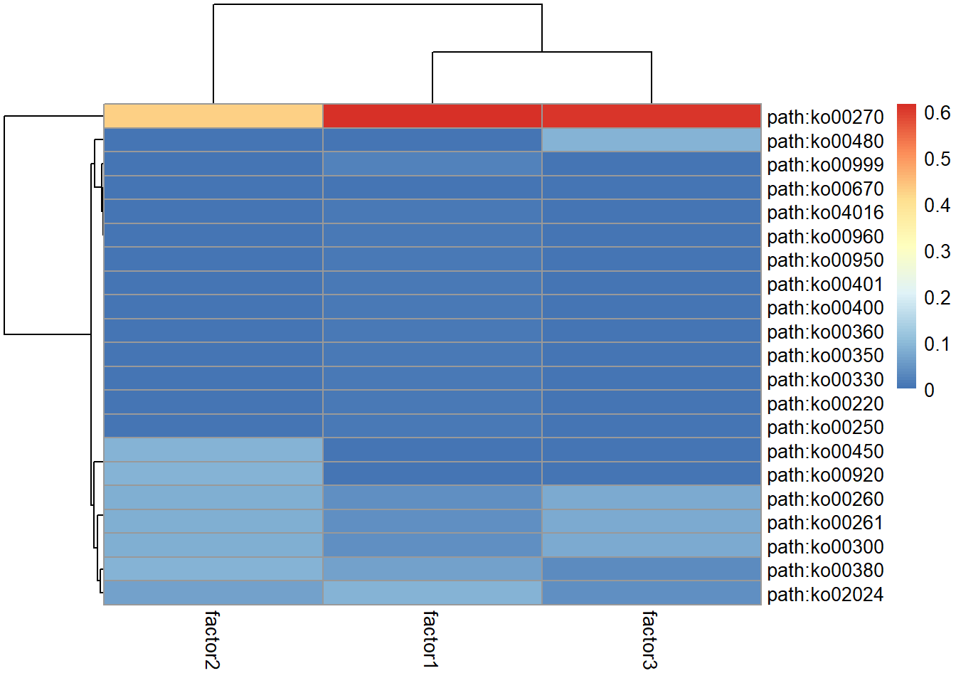

These information can be further combined with the other functions in stana, like plotting factor profiles along with the tree inferred from consensus sequence alignment, linking allele frequency information and gene copy number data.

ab <- plotAbundanceWithinSpecies(stana, "100003", tss=TRUE, return_data=TRUE)
stana <- setMetadata(stana, ab)
stana <- inferAndPlotTree(stana, "100003", meta=colnames(ab))
getTreePlot(stana)
#> $`100003`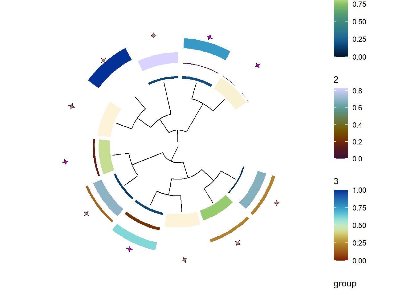

3.2.1 Scaling function for NNLM

As same as scale function in NMF, the helper function for NNLM resulting object is prepared (scaler.NNLM).

3.3 PERMANOVA

Using adonis2 function in vegan, one can compare distance matrix based on SNV frequency or gene (gene family) copy numbers, or tree-based distance between the specified group. When the target="tree" is specified, tree shuold be in treeList, with the species name as the key. The ape::cophenetic.phylo() is used to calculate distance between tips based on branch length. Distance method can be chosen from dist function in stats, and the default is set to manhattan. You can specify distArg to pass the arguments to dist. Also, the distance calculated directly from sequences can be used. In this case, target='fasta' should be chosen, and the function to calculate distance should be provided to AAfunc argument.

stana <- setTree(stana, "100003", tre)
stana <- doAdonis(stana, specs = "100003", target="tree")
#> # Performing adonis in 100003 target is tree
#> #  F: 0.719649945825046, R2: 0.0740407267582885, Pr: 0.695
getAdonis(stana)[["100003"]]
#> Permutation test for adonis under reduced model
#> Permutation: free
#> Number of permutations: 999
#> 
#> adonis2(formula = d ~ ., data = structure(list(group = c("Group1", "Group1", "Group1", "Group1", "Group2", "Group2", "Group2", "Group2", "Group2", "Group2", "Group2")), row.names = c("ERR1711593", "ERR1711594", "ERR1711596", "ERR1711598", "ERR1711603", "ERR1711605", "ERR1711606", "ERR1711609", "ERR1711611", "ERR1711612", "ERR1711618"), class = "data.frame"))
#>          Df SumOfSqs      R2      F Pr(>F)
#> Model     1  0.15557 0.07404 0.7196  0.695
#> Residual  9  1.94558 0.92596              
#> Total    10  2.10115 1.00000

The corresponding principal coordinate analysis plot using distance matrix can be drawn by specifying pcoa. The relative eigenvalues are plotted.

stana <- doAdonis(stana, specs = "100003",
    target="genes", pcoa=TRUE)
#> # Performing adonis in 100003 target is genes
#> #  F: 0.950009752773493, R2: 0.0635457614064265, Pr: 0.578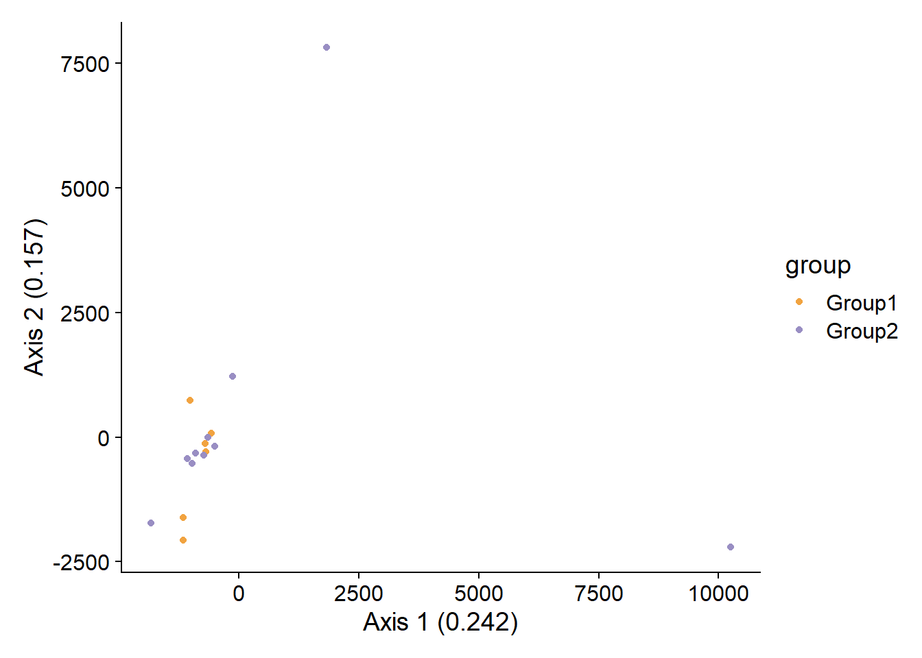

By default, the function uses grouping variable in cl slot. For more complex modeling, the slot meta can be populated by the data frame of samples by setMetadata like the example below. To use metadata, useMeta option should be specified with the formula argument.

stana <- doAdonis(stana, specs = "100003",
    target="genes", useMeta=TRUE, formula = "d ~ .")
#> # Performing adonis in 100003 target is genes
#> # Printing raw adonis results ...
#> No residual component
#> 
#> adonis2(formula = d ~ ., data = structure(list(`1` = c(0.985829902295573, 0.852470142666385, 0.194983622925863, 0.1702484777323, 0, 0.01749079304296, 0.169551265957738, 1, 0.774981822424855, 0, 0, 1, 0.145056521442649, 0.894711680596164, 0.725364565076885, 0.0951555820116268), `2` = c(0.0141700977044264, 0.147529857333615, 0.0484882264088995, 0.221175192027691, 1, 0.98250920695704, 0.830448734042262, 0, 0, 0.911065650363313, 0, 0, 0.693043447598221, 0.0456195965920271, 0.274635434923115, 0.67607988474988
#>          Df  SumOfSqs R2 F Pr(>F)
#> Model    15 501125509  1         
#> Residual  0         0  0         
#> Total    15 501125509  1
getAdonis(stana)[["100003"]]
#> No residual component
#> 
#> adonis2(formula = d ~ ., data = structure(list(`1` = c(0.985829902295573, 0.852470142666385, 0.194983622925863, 0.1702484777323, 0, 0.01749079304296, 0.169551265957738, 1, 0.774981822424855, 0, 0, 1, 0.145056521442649, 0.894711680596164, 0.725364565076885, 0.0951555820116268), `2` = c(0.0141700977044264, 0.147529857333615, 0.0484882264088995, 0.221175192027691, 1, 0.98250920695704, 0.830448734042262, 0, 0, 0.911065650363313, 0, 0, 0.693043447598221, 0.0456195965920271, 0.274635434923115, 0.67607988474988
#>          Df  SumOfSqs R2 F Pr(>F)
#> Model    15 501125509  1         
#> Residual  0         0  0         
#> Total    15 501125509  1

3.4 Comparing gene copy numbers

If you have genes slot filled in the stana object, gene copy numbers can be compared one by one using exact Wilcoxon rank-sum test using wilcox.exact in exactRankTests computing exact conditional p-values. Note that p-values are not adjusted for multiple comparisons made.

res <- compareGenes(stana, "100003")
#> # Testing total of 21806
res[["UHGG000008_01733"]]
#> 
#>  Exact Wilcoxon rank sum test
#> 
#> data:  c(1.154444, 2.404241, 0, 1.421386, 1.50773, 0) and c(0.535732, 1.709442, 1.31675, 3.44086, 2.712423, 1.923076, 1.062853, c(1.154444, 2.404241, 0, 1.421386, 1.50773, 0) and 1.21147, 0, 1.509217)
#> W = 22, p-value = 0.4256
#> alternative hypothesis: true mu is not equal to 0

3.5 Aggregating gene copy numbers

The gene copy numbers across multiple stana object can be aggregated. This returns the new stana object where the gene copy numbers are combined.

## This returns new stana object
stanacomb <- combineGenes(list(stana, stana), species="100003")
#> Common genes: 21806
#> Duplicate label found in group
dim(getSlot(stanacomb, "genes")[["100003"]])
#> [1] 21806    32

3.6 Performing Boruta or feature selection

Boruta algorithm can be run on matrices to obtain important marker (SNV position or gene) for distinguishing between group by doBoruta function. The function performs Boruta algorithm on specified data and returns the Boruta class result. By default, the function performs fixes to tentative input. To disable this, specify doFix=FALSE.

library(Boruta)
brres <- doBoruta(stana, "100003")
#> # Using grouping from the slot: Group1/Group2
#> # If needed, please provide preprocessed matrix to `mat`
#> # Feature number: 21806
#> # Performing Boruta
brres
#> $boruta
#> Boruta performed 99 iterations in 27.66723 secs.
#> Tentatives roughfixed over the last 99 iterations.
#>  15 attributes confirmed important: UHGG000008_01798,
#> UHGG004375_00184, UHGG025024_01181, UHGG061776_01339,
#> UHGG155301_01986 and 10 more;
#>  21791 attributes confirmed unimportant:
#> UHGG000008_00008, UHGG000008_00009, UHGG000008_00010,
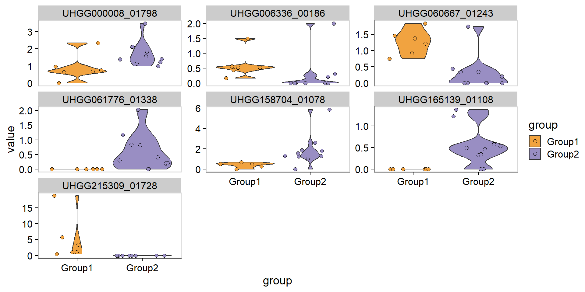
#> UHGG000008_00012, UHGG000008_00015 and 21786 more;

Further, we visualize the copy numbers of important genes confirmed between the group.

confirmed_genes <- brres$boruta$finalDecision[brres$boruta$finalDecision=="Confirmed"] %>% names()
plotGenes(stana, "100003", confirmed_genes)+
  ggplot2::facet_wrap(.~geneID,scales="free_y")+
  cowplot::theme_cowplot() +
  cowplot::panel_border()