2 Importing and filtering
stana is aimed to import the metagenotyping results of various pipelines.
The package is designed to handle some types of the metagenotyping software such as MIDAS and MIDAS2, which outputs the
gene copy numbers by default. Note that the slot name snps here refers to just the variable, and not to reflect the actual meaning. The species ID in stana object is interpreted as character.
library(stana)Along with specifying which directory to load, the grouping variables should be set to stana object. By default, named list of groups is used (categorical). The cl argument in the functions and cl slot corresponds to this information. Additionally, the metadata in ordinaly data.frame can be set by setMetadata. The row names or id column should represent the sample names.
If species IDs are not specified, all the species in the directory will be loaded, which consumes many times and memory if the sample number is large.
2.1 MIDAS
For MIDAS, loadMIDAS function can be used to import the output of merge command. In MIDAS and MIDAS2 examples, we load the example dataset deposited by the study investigating gut microbiome of hemodialysis patients (Shi et al. 2022). hd_meta includes named list of grouping. First we would like to see how many samples were profiled in the species.
load("../hd_meta.rda")
stana <- loadMIDAS("../merge_midas1", cl=hd_meta, only_stat=TRUE)
stana$snps |> head() |> DT::datatable()
We will load the interesting species.
stana <- loadMIDAS("../merge_midas1/", cl=hd_meta, candSp="Bacteroides_uniformis_57318")
#> Bacteroides_uniformis_57318
#>   Snps
#>     HC 13
#>     R 16
#>     Bacteroides_uniformis_57318 cleared filtering threshold in SNV
#>   Genes
#>     HC 13
#>     R 16
#>     Bacteroides_uniformis_57318 cleared filtering threshold in genes
#> Overall, 1 species met criteria in SNPs
#> Overall, 1 species met criteria in genes
stana
#> # A stana: MIDAS1
#> # Loaded directory: ../merge_midas1/
#> # Species number: 1
#> # Group info (list): HC/R
#> # Loaded SNV table: 1 ID: Bacteroides_uniformis_57318
#> # Loaded gene table: 1 ID: Bacteroides_uniformis_57318
#> # Size: 14.586864 MB
2.2 MIDAS2
For MIDAS2, loadMIDAS2 function can be used to import the output of merge command.
For MIDAS2, the function assumes the default database of UHGG or GTDB is used. For the other custom databases, use snv and gene function described in this documentation.
For MIDAS2, the lz4 binary must be in PATH to correctly load the data.
load("../hd_meta.rda")
hd_meta
#> $HC
#>  [1] "ERR9492498" "ERR9492502" "ERR9492507" "ERR9492508"
#>  [5] "ERR9492512" "ERR9492497" "ERR9492499" "ERR9492501"
#>  [9] "ERR9492504" "ERR9492505" "ERR9492509" "ERR9492511"
#> [13] "ERR9492500" "ERR9492503" "ERR9492506" "ERR9492510"
#>
#> $R
#>  [1] "ERR9492489" "ERR9492490" "ERR9492492" "ERR9492494"
#>  [5] "ERR9492519" "ERR9492524" "ERR9492526" "ERR9492527"
#>  [9] "ERR9492528" "ERR9492513" "ERR9492514" "ERR9492518"
#> [13] "ERR9492520" "ERR9492522" "ERR9492523" "ERR9492525"
#> [17] "ERR9492491" "ERR9492493" "ERR9492495" "ERR9492496"
#> [21] "ERR9492515" "ERR9492516" "ERR9492517" "ERR9492521"
We can check stats of how many samples are profiled for each species, by only_stat. This returns the list of tibbles with names snps and genes.
stana <- loadMIDAS2("../merge_uhgg", only_stat=TRUE, cl=hd_meta)
stana$snps |> dplyr::filter(group=="HC") |> dplyr::arrange(desc(n)) |> head()
#> # A tibble: 6 × 5
#> # Groups:   species_id [6]
#>   species_id group     n species_name    species_description
#>   <chr>      <chr> <int> <chr>           <chr>
#> 1 101346     HC       12 s__KS41 sp0035… s__KS41 sp003584895
#> 2 102438     HC       10 s__Synechococc… s__Synechococcus_C…
#> 3 101378     HC        9 s__CAG-873 sp0… s__CAG-873 sp00249…
#> 4 102478     HC        9 s__Clostridium… s__Clostridium_A l…
#> 5 102492     HC        8 s__Thalassospi… s__Thalassospira l…
#> 6 100044     HC        7 s__Helicobacte… s__Helicobacter py…
As the long output is expected, only one species is loaded here.
stana <- loadMIDAS2("../merge_uhgg", candSp="100002", cl=hd_meta)
#>   100002
#>   s__Staphylococcus aureus
#>     Number of snps: 2058
#>     Number of samples: 5
#>   100002
#>   s__Staphylococcus aureus
#>     Number of genes: 23427
#>     Number of samples: 7
The data is profiled against UHGG. loadSummary and loadInfo can be specified to load the SNV summary and SNV info per species, which is default to TRUE.
getSlot(stana, "snps")[["100002"]] |> head()
#>                                 ERR9492497 ERR9492515
#> gnl|Prokka|UHGG000004_1|2901|A           1          1
#> gnl|Prokka|UHGG000004_1|4071|C           1          0
#> gnl|Prokka|UHGG000004_1|11094|T          1          0
#> gnl|Prokka|UHGG000004_1|11148|T          1          0
#> gnl|Prokka|UHGG000004_1|11940|G          0          0
#> gnl|Prokka|UHGG000004_1|11970|C          0          0
#>                                 ERR9492526 ERR9492527
#> gnl|Prokka|UHGG000004_1|2901|A           0      0.429
#> gnl|Prokka|UHGG000004_1|4071|C           1      0.000
#> gnl|Prokka|UHGG000004_1|11094|T          0      0.000
#> gnl|Prokka|UHGG000004_1|11148|T          0      0.429
#> gnl|Prokka|UHGG000004_1|11940|G          1      0.444
#> gnl|Prokka|UHGG000004_1|11970|C          1      0.556
#>                                 ERR9492528
#> gnl|Prokka|UHGG000004_1|2901|A           0
#> gnl|Prokka|UHGG000004_1|4071|C           0
#> gnl|Prokka|UHGG000004_1|11094|T          1
#> gnl|Prokka|UHGG000004_1|11148|T          1
#> gnl|Prokka|UHGG000004_1|11940|G          0
#> gnl|Prokka|UHGG000004_1|11970|C          0
getSlot(stana, "freqTableSnps") |> head()
#> data frame with 0 columns and 0 rows
By default, the taxonomy ID will be converted using the default MIDAS2 database information.
The coverage for each species per sample is plotted by plotCoverage.
plotCoverage(stana, "100002", pointSize=5)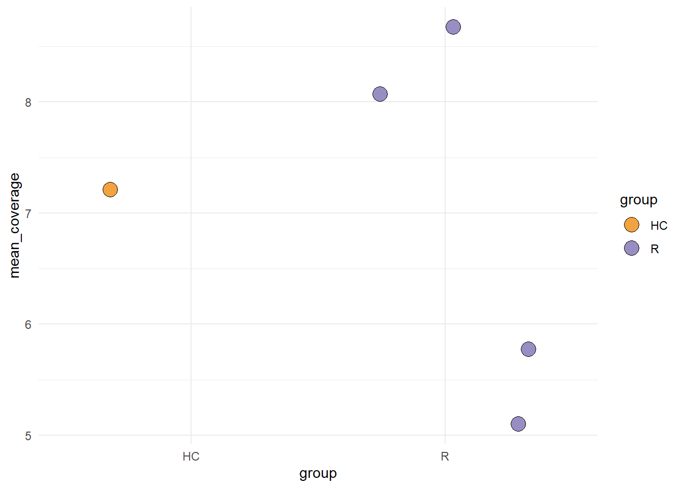
2.3 inStrain
For inStrain, we need compare command output, after profile command. First we would like to know which species are profiled. just_species option only list species in the table. Here, we load an example dataset profiled by inStrain, using the default database described in their original tutorial. For inStrain, loading all the SNV tables is often impossible, we must specify candidate_species for investigation.
sp <- loadInStrain("../inStrain_out", just_species=TRUE)
sp
#>  [1] "GUT_GENOME000022" "GUT_GENOME000024"
#>  [3] "GUT_GENOME000147" "GUT_GENOME000220"
#>  [5] "GUT_GENOME000221" "GUT_GENOME000224"
#>  [7] "GUT_GENOME000225" "GUT_GENOME000231"
#>  [9] "GUT_GENOME000509" "GUT_GENOME007566"
#> [11] "GUT_GENOME009103" "GUT_GENOME031782"
#> [13] "GUT_GENOME034989" "GUT_GENOME044231"
#> [15] "GUT_GENOME067546" "GUT_GENOME068725"
#> [17] "GUT_GENOME080972" "GUT_GENOME090701"
#> [19] "GUT_GENOME094995" "GUT_GENOME096045"
#> [21] "GUT_GENOME096080" "GUT_GENOME096083"
#> [23] "GUT_GENOME096473" "GUT_GENOME096573"
#> [25] "GUT_GENOME102034" "GUT_GENOME103721"
#> [27] "GUT_GENOME104570" "GUT_GENOME109880"
#> [29] "GUT_GENOME112794" "GUT_GENOME113322"
#> [31] "GUT_GENOME114679" "GUT_GENOME115272"
#> [33] "GUT_GENOME115357" "GUT_GENOME116258"
#> [35] "GUT_GENOME116897" "GUT_GENOME117271"
#> [37] "GUT_GENOME132077" "GUT_GENOME135463"
#> [39] "GUT_GENOME140076" "GUT_GENOME142015"
#> [41] "GUT_GENOME142390" "GUT_GENOME143131"
#> [43] "GUT_GENOME143211" "GUT_GENOME143348"
#> [45] "GUT_GENOME143497" "GUT_GENOME143505"
#> [47] "GUT_GENOME149497" "GUT_GENOME156849"
#> [49] "GUT_GENOME174809" "GUT_GENOME175554"
#> [51] "GUT_GENOME189814" "GUT_GENOME195293"
#> [53] "GUT_GENOME208589" "GUT_GENOME210309"
#> [55] "GUT_GENOME210710" "GUT_GENOME217823"
#> [57] "GUT_GENOME217842" "GUT_GENOME217850"
#> [59] "GUT_GENOME234840" "GUT_GENOME252930"
#> [61] "GUT_GENOME258721" "GUT_GENOME261411"
#> [63] "GUT_GENOME272874" "GUT_GENOME274362"
#> [65] "GUT_GENOME275708" "GUT_GENOME277090"
#> [67] "GUT_GENOME284693" "GUT_GENOME286118"
This recalculates the minor allele frequency based on pooled SNV information (not on individual SNV information), thus takes a long time in case the number of profiled positions is large. We can set cl argument if needed.
instr_chk <- "GUT_GENOME142015"
instr <- loadInStrain("../inStrain_out", instr_chk, skip_pool=FALSE) ## Load MAF table
#> Loading allele count table
#> Loading the large table...
#> Loading key table
#> Loading info table
#> Candidate species: GUT_GENOME142015
#>   Candidate key numbers: 1
#>   Dimension of pooled SNV table for species: 2359827
#> Calculating MAF
instr
#> # A stana: InStrain
#> # Loaded directory: ../inStrain_out
#> # Species number: 1
#> # Loaded SNV table: 1 ID: GUT_GENOME142015
#> # Size: 82.902808 MB
2.4 metaSNV
For loading the output of metaSNV, metaSNV.py and metaSNV_Filtering.py are typically performed beforehand. You can use just_species to return species ID. Note that the loadmetaSNV is currently supported to load only the SNV profiles.
meta <- loadmetaSNV("../metasnv_sample_out")
#>   Loading refGenome1clus
#>   Loading refGenome2clus
#>   Loading refGenome3clus
2.5 Manual
The loading of the manually created data.frame is possible by snv, gene, GF functions, each prepared for SNV, gene copy numbers, and gene family copy number tables. The metagenotyping results produced by the other software can be loaded with this function, although some statistics should be inserted manually. These functions accepts the named list of data.frame. If the software like HUMAnN3 is used to profile the functional implications from metagenomic reads, the subset stratified output can also be used for GF function.
man <- snv(list("manual"=head(getSlot(meta, "snps")[[1]])))
man
#> # A stana: manual
#> # Loaded directory:
#> # Species number: 1
#> # Loaded SNV table: 1 ID: manual
#> # Size: 0.050072 MB
## HUMAnN merged profile
df <- read.table("humann_merged_ko_eval_45.txt", sep="\t", header=1, row.names=1, check.names=FALSE, comment.char = "")
stana <- fromHumann(df)
stana
#> # A stana: manual
#> # Loaded directory:
#> # Species number: 344
#> # Loaded KO table: 344 ID: g__Bifidobacterium.s__Bifidobacterium_longum
#> # Size: 37.921952 MB
2.5.1 Conversion to MAF matrix
Some metagenotype data comes with TSV with the number of allele count with long or wide format. The package offers some functions to convert these to MAF matrix.
df1 <- data.frame(rbind(
  c("SPID1","SP1_NZ_GG770218.1_131457", "G", "A", "7", "2"),
  c("SPID1","SP1_NZ_GG770218.1_131458", "C", "T", "2", "5"),
  c("SPID2","SP2_NZ.1_131459", "A", "T", "7", "13"),
  c("SPID2","SP2_NZ.1_131470", "A", "T", "12", "2")
))

head(df1)
#>      X1                       X2 X3 X4 X5 X6
#> 1 SPID1 SP1_NZ_GG770218.1_131457  G  A  7  2
#> 2 SPID1 SP1_NZ_GG770218.1_131458  C  T  2  5
#> 3 SPID2          SP2_NZ.1_131459  A  T  7 13
#> 4 SPID2          SP2_NZ.1_131470  A  T 12  2

convertWideToMaf(df1)[[1]]
#> $SPID1
#>                                maf
#> SP1_NZ_GG770218.1_131457 0.2222222
#> SP1_NZ_GG770218.1_131458 0.2857143
#>
#> $SPID2
#>                       maf
#> SP2_NZ.1_131459 0.3500000
#> SP2_NZ.1_131470 0.1428571


df2 <- data.frame(rbind(
  c("SPID3","SP3_AZ.1_131457", "G", "A", "7", "2"),
  c("SPID3","SP3_AZ.1_131458", "C", "T", "2", "5"),
  c("SPID1","SP1_NZ_GG770218.1_131457", "A", "T", "7", "13"),
  c("SPID1","SP1_NZ_GG770218.1_131458", "A", "T", "12", "2")
))
They can be merged to make stana object by combineMaf() function.
mafs <- list("sample1"=convertWideToMaf(df1), "sample2"=convertWideToMaf(df2))
stana <- combineMaf(mafs)
stana
#> # A stana: manual
#> # Loaded directory:
#> # Species number: 0
#> # Loaded SNV table: 3 ID: SPID1
#> # Size: 0.024008 MB
getSlot(stana, "snpsInfo")
#> [[1]]
#>                           major_allele minor_allele
#> SP1_NZ_GG770218.1_131457             G            A
#> SP1_NZ_GG770218.1_131458             T            C
#> SP1_NZ_GG770218.1_1314571            T            A
#> SP1_NZ_GG770218.1_1314581            A            T
#>                           species_id sample_name
#> SP1_NZ_GG770218.1_131457       SPID1     sample1
#> SP1_NZ_GG770218.1_131458       SPID1     sample1
#> SP1_NZ_GG770218.1_1314571      SPID1     sample2
#> SP1_NZ_GG770218.1_1314581      SPID1     sample2
#>
#> [[2]]
#>                 major_allele minor_allele species_id
#> SP2_NZ.1_131459            T            A      SPID2
#> SP2_NZ.1_131470            A            T      SPID2
#>                 sample_name
#> SP2_NZ.1_131459     sample1
#> SP2_NZ.1_131470     sample1
#>
#> [[3]]
#>                 major_allele minor_allele species_id
#> SP3_AZ.1_131457            G            A      SPID3
#> SP3_AZ.1_131458            T            C      SPID3
#>                 sample_name
#> SP3_AZ.1_131457     sample2
#> SP3_AZ.1_131458     sample2

## If needed, SNV-level statistics should be set to stana
# stana <- setSlot(stana, "snpsSummary", summary_df)
This object can be used with the subsequent downstream analysis. The function can be useful in importing the metagenotyping software such as GT-Pro.
2.6 Filtering by species ID
The check method applied to stana object can check the samples or species met the specific criteria.
stana <- loadMIDAS2("../merge_uhgg", cl=hd_meta, candSp="100002", db="uhgg")
#>   100002
#>   g__Blautia_A;s__Blautia_A sp900066165
#>     Number of snps: 2058
#>     Number of samples: 5
#>   100002
#>   g__Blautia_A;s__Blautia_A sp900066165
#>     Number of genes: 23427
#>     Number of samples: 7
filt <- stana %>% check(mean_coverage > 4)
head(filt %>% dplyr::arrange(dplyr::desc(n)))
#> # A tibble: 6 × 3
#>   species_id     n species_description
#>        <int> <int> <chr>
#> 1     102478    31 g__Bacteroides_B;s__Bacteroides_B dorei
#> 2     101346    28 g__Bacteroides;s__Bacteroides uniformis
#> 3     102438    28 g__Parabacteroides;s__Parabacteroides di…
#> 4     100074    21 g__Alistipes;s__Alistipes onderdonkii
#> 5     100044    20 g__Parabacteroides;s__Parabacteroides me…
#> 6     101338    19 g__Blautia_A;s__Blautia_A wexlerae
Subsequently, filter method can be used to subset the stana object for interesting species.
Most of the functions in stana is designed to perform the analysis in all the species within stana object unless specified, so the filtering beforehand with grouping variables is important (such as number of samples profiled per group).
2.7 Filtering the site IDs for the SNV
The users can preset the SNV ID used for the downstream calculation to the includeSNVID slot in the stana object. When this information is used, the function raises the message that it is using the IDs.
stana <- siteFilter(stana, getID(stana)[1], site_type=="4D")
#> # total of 650 obtained from 2058
## Downstream functions use the filtered site IDs2.8 Printing the profile information
By show or print method, the summary of stana object is outputted.
Also, summary method can be used to inspect the grouping information per species.
stana
#> # A stana: MIDAS2
#> # Database: uhgg
#> # Loaded directory: ../merge_uhgg
#> # Species number: 1
#> # Group info (list): HC/R
#> # Loaded SNV table: 1 ID: 100002
#> # Loaded gene table: 1 ID: 100002
#> # Size: 4.527176 MB
summary(stana)
#> #
#> # SNV description
#> # A tibble: 2 × 3
#> # Groups:   group [2]
#>   group species_id                                n
#>   <chr> <chr>                                 <int>
#> 1 HC    g__Blautia_A;s__Blautia_A sp900066165     1
#> 2 R     g__Blautia_A;s__Blautia_A sp900066165     4
#> # Gene description
#> # A tibble: 2 × 3
#> # Groups:   group [2]
#>   group species_id                                n
#>   <chr> <chr>                                 <int>
#> 1 HC    g__Blautia_A;s__Blautia_A sp900066165     1
#> 2 R     g__Blautia_A;s__Blautia_A sp900066165     6