3 Penalized regressions
Penalized regression is a type of regression analysis that includes a penalty term to prevent overfitting and improve the generalizability of the model. It is particularly useful when dealing with high-dimensional data where the number of predictors is large compared to the number of observations. In terms of inference of GRN and BN structure learning, the penalized regression has been used successfully (Schmidt, Niculescu-Mizil, and Murphy 2007). The package implments the core algorithms for the use of penalization in the BN structure learning described below.
3.1 Algorithms
3.1.1 glmnet_BIC and glmnet_CV
For L1 regularization (LASSO), the package uses the popular R library glmnet. The glmnet_BIC specified in the argument algo will select the lambda by the minimum BIC criteria, while the glmnet_CV choose the lambda based on cross validation with the specified fold numbers. glmnetBICpath returns the BIC path given the data.frame and the node name to be modeled. plot contains the BIC path plot, and fit contains the fitted object and BIC the lambda and BIC data.frame. The maximize function can be chosen by maximize argument in algorithm.args list. Greedy Equivalence Search can be performed via setting this argument to ges.
library(scran)
library(scstruc)
library(bnlearn)

sce <- mockSCE()
sce <- logNormCounts(sce)
included_genes <- sample(row.names(sce), 30)

## Inference based on glmnet_CV and maximization by GES
gs <- scstruc(sce, included_genes,
    algorithm="glmnet_CV",
    algorithm.args=list("maximize"="ges"),
    changeSymbol=FALSE)
gs$net
#>
#>   Random/Generated Bayesian network
#>
#>   model:
#>    [Gene_0023][Gene_0145][Gene_0156][Gene_0425][Gene_0544]
#>    [Gene_0725][Gene_0814][Gene_0993][Gene_1085][Gene_1214]
#>    [Gene_1267][Gene_1292][Gene_1330][Gene_1332][Gene_1375]
#>    [Gene_1569][Gene_1683][Gene_1700][Gene_1744][Gene_1922]
#>    [Gene_2000][Gene_0348|Gene_1085:Gene_1700]
#>    [Gene_0863|Gene_0425][Gene_1091|Gene_0814]
#>    [Gene_1520|Gene_0425][Gene_0118|Gene_0348]
#>    [Gene_0887|Gene_0348][Gene_1921|Gene_0863:Gene_1700]
#>    [Gene_0986|Gene_0887][Gene_1541|Gene_1921:Gene_2000]
#>   nodes:                                 30
#>   arcs:                                  12
#>     undirected arcs:                     0
#>     directed arcs:                       12
#>   average markov blanket size:           1.00
#>   average neighbourhood size:            0.80
#>   average branching factor:              0.40
#>
#>   generation algorithm:                  Empty

## Visualization of glmnet_BIC criteria
## Just to obtain data to be used in the inference
gs <- scstruc(sce, included_genes,
    changeSymbol=FALSE, returnData=TRUE)

set.seed(10)
glmnetBICpath(gs$data, sample(colnames(gs$data), 1))[["plot"]]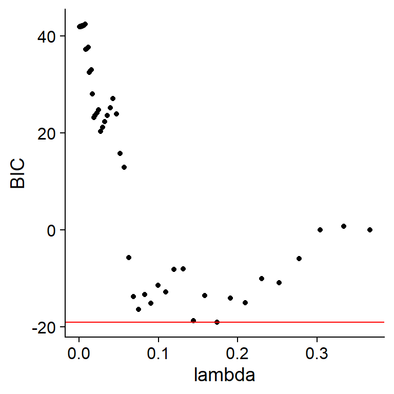
3.1.2 MCP_CV and SCAD_CV
Same as glmnet_CV, the library performs penalized regression baed on MCP and SCAD using ncvreg library.
library(ncvreg)

mcp.net <- scstruc(sce, included_genes,
    algorithm="MCP_CV", returnData=FALSE,
    changeSymbol=FALSE)

scad.net <- scstruc(sce, included_genes,
    algorithm="SCAD_CV", returnData=FALSE,
    changeSymbol=FALSE)

## Using the bnlearn function to compare two networks
bnlearn::compare(mcp.net, scad.net)
#> $tp
#> [1] 6
#>
#> $fp
#> [1] 4
#>
#> $fn
#> [1] 0
3.1.3 L0-regularized regression
Based on the L0Learn, the package performs structure learning based on L0-regularized regression. L0 regularization, also known as best subset selection, is a technique used to build simpler and more interpretable models by selecting only a small number of important variables. L0L1 and L0L2 regularization is a combination of L0, L1, and L2 regularization. For the details of L0-, L0L1-, or L0L2-regularized regression, please consult the original paper (Hazimeh, Mazumder, and Nonet 2023).
l0l2.net <- scstruc(sce, included_genes,
    algorithm="L0L2_CV", returnData=FALSE,
    changeSymbol=FALSE)
plotNet(l0l2.net)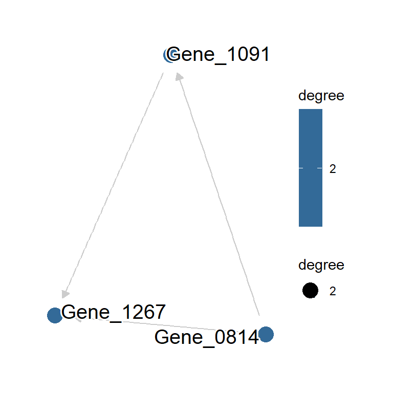
3.1.4 CCDr algorithm
Generally, the CCDr algorithm is the fastest algorithm and learns the network for multiple lambdas. By default, the function chooses the network with the best BIC value among multiple lambdas. To supress this effect and obtain all networks, set bestScore to FALSE in the algorithm.args.
library(ccdrAlgorithm);library(sparsebnUtils)
ccdr.res <- scstruc(sce, included_genes,
    algorithm="ccdr", changeSymbol=FALSE,
    algorithm.args=list(bestScore=FALSE))
#> Setting `lambdas.length` to 10
#> Returning the bn per lambda from result of ccdr.run
names(ccdr.res$net)
#> [1] "14.1421356237309"  "8.47798757230114"
#> [3] "5.08242002399425"  "3.04683075789017"
#> [5] "1.82652705274248"  "1.09497420090059"
#> [7] "0.656419787945471" "0.393513324471009"
ccdr.res$net[[4]]
#>
#>   Random/Generated Bayesian network
#>
#>   model:
#>    [Gene_0023][Gene_0118][Gene_0145][Gene_0156][Gene_0425]
#>    [Gene_0544][Gene_0725][Gene_0814][Gene_0887][Gene_0986]
#>    [Gene_0993][Gene_1085][Gene_1091][Gene_1214][Gene_1267]
#>    [Gene_1292][Gene_1330][Gene_1332][Gene_1375][Gene_1520]
#>    [Gene_1541][Gene_1569][Gene_1683][Gene_1700][Gene_1744]
#>    [Gene_1921][Gene_1922][Gene_2000][Gene_0348|Gene_0118]
#>    [Gene_0863|Gene_0425]
#>   nodes:                                 30
#>   arcs:                                  2
#>     undirected arcs:                     0
#>     directed arcs:                       2
#>   average markov blanket size:           0.13
#>   average neighbourhood size:            0.13
#>   average branching factor:              0.067
#>
#>   generation algorithm:                  Empty
Therefore, the bootstrap-based inference can be performed very fast using CCDr algorithm. If bootstrapping is specified, the function performs learning the bootstrapped network for the multiple lambdas across all the replicates.
3.1.5 Precision lasso
Precision Lasso combines the LASSO and the precision matrix into the regularization process. This approach is particularly useful in biological and genomics studies, where highly-correlated features often appear. We implmented precision lasso in R and the feature is provided by plasso.fit and plasso.fit.single using RcppArmadillo. The fixed lambda value should be specified.
pl.res <- scstruc(sce, included_genes, algorithm="plasso", changeSymbol=FALSE)