6 Evaluating the inferred networks
For the interpretation of the results, the assessment of inferred networks is crucial. This is because it is necessary to determine which network should be used for downstream analysis, and to assess how closely the inferred causal relationships resemble those of biologically validated networks. One of the core features of the scstruc is evaluating and selecting optimal algorithms from the inferred networks. We describe how to evaluate the inferred networks using various metrics in this section. The implemented metrics include:
- True positive arcs
- False positive arcs
- False negative arcs
- Precision
- Recall
- F1-score
- Bayesian Information Criterion (if the data to be fitted is provided)
- Structural Hamming Distance
- Structural Intervention Distance (with or without symmetrization)
- Kullback–Leibler divergence
- AUPRC (for bootstrapped network only)
6.1 Evaluation functions
6.1.1 metrics function
This function accepts learned networks and the reference network (both should be bn object) and outputs data.frame consisting of various metrics.
library(scstruc)
net <- readRDS("ecoli70.rds")
data.inference <- rbn(net, 50)
infer <- hc(data.inference)
metrics(bn.net(net), list("inferred"=infer))
#>       algo referenceNode InferenceNode s0 edges SHD TP FP
#> 1 inferred            46            46 70    99 107 28 42
#>   FN TPR Precision    Recall        F1 SID KL BIC
#> 1 71 0.4       0.4 0.2828283 0.3313609 958 NA  NA
sid_sym argument can choose whether to symmetrze the SID, and SID.cran can choose whether to use SID implemented in CRAN package SID.
6.1.2 metricsFromFitted function
This function accepts parameter-fitted network and sampling number, as well as the algorithms to be used in the inference. Using rbn function in bnlearn, logic sampling is performed from fitted network. Here, we use ECOLI70 network from GeneNet R package, sampling 50 observations from the network. The testing algorithms can be specifed by argument algos. For the special algorithms, the arguments with the same name are provided. The function has return_data and return_net argument, which returns the data used in the inference and inferred networks. By default, only the metrics is returned.
mf <- metricsFromFitted(net, 50, algos=c("glmnet_CV", "glmnet_BIC", "L0_CV"))
#> glmnet_CV 5.95810103416443
#> glmnet_BIC 0.471029996871948
#> L0_CV
#> 5.5213348865509
#> MMHC 0.001 0.0360720157623291
#> MMHC 0.005 0.0354738235473633
#> MMHC 0.01 0.0376400947570801
#> MMHC 0.05 0.0452709197998047
#> Network computing finished
head(mf$metrics)
#>         algo s0 edges        KL       BIC SHD TP FP FN
#> 1  glmnet_CV 70    68  5.145568 -2347.568  69 31 39 37
#> 2 glmnet_BIC 70    38 14.594425 -2508.020  55 23 47 15
#> 3      L0_CV 70    30 64.437907 -2893.720  67 13 57 17
#> 4 mmhc_0.001 70    26 54.579934 -2797.366  59 15 55 11
#> 5 mmhc_0.005 70    28 44.462021 -2747.934  60 16 54 12
#> 6  mmhc_0.01 70    29 43.507040 -2728.172  59 17 53 12
#>         TPR Precision    Recall        F1 SID PPI
#> 1 0.4428571 0.4428571 0.4558824 0.4492754  NA  NA
#> 2 0.3285714 0.3285714 0.6052632 0.4259259  NA  NA
#> 3 0.1857143 0.1857143 0.4333333 0.2600000  NA  NA
#> 4 0.2142857 0.2142857 0.5769231 0.3125000  NA  NA
#> 5 0.2285714 0.2285714 0.5714286 0.3265306  NA  NA
#> 6 0.2428571 0.2428571 0.5862069 0.3434343  NA  NA
#>         time   BICnorm  N  p
#> 1 5.95810103 1.0000000 50 46
#> 2 0.47103000 0.8938548 50 46
#> 3 5.52133489 0.6387000 50 46
#> 4 0.03607202 0.7024417 50 46
#> 5 0.03547382 0.7351427 50 46
#> 6 0.03764009 0.7482163 50 46
The results can be visualized in the usual way by using the library like ggplot2. We use here plotthis library for visualizing.
library(plotthis)
library(ggplot2)
library(ggrepel)
ScatterPlot(mf$metrics, x="SHD", y="F1", color_by="algo", legend.position="none") +
    geom_text_repel(aes(label=algo), bg.colour="white")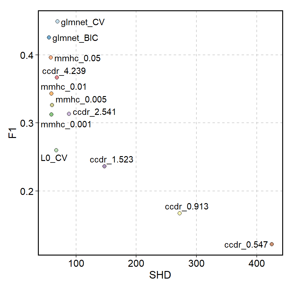
6.2 Evaluating the causal validity
The primary objective of the package is evaluating the causal validity of the inferred networks. Two approach can be used, in the situations that the reference directed network is available or not. In most of the cases, the reference networks is not readily available.
6.2.1 Obtaining the directed acyclic graphs (DAGs) for the evaluation
For the interesting biological pathway, one can obtain DAG from the KEGG PATHWAY. The getKEGGEdges function accepts the pathway identifier and returns the DAG, though it will not always succeed. The function first parses the pathway information using ggkegg, and identify the largest components to be evaluated. If removeCycle is TRUE, the function identifies the minimum feedback using igraph function and remove these edges. This returns the bn object.
Suppose you are interested in inferring gene regulatory networks in mTOR signaling pathway from your dataset, you should first load DAG from the KEGG API.
library(scstruc)
dags <- getKEGGEdges("mmu04150", removeCycle=TRUE)
#> Removing Pik3ca|Mtor
graphviz.plot(dags)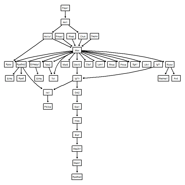
Using the genes in this candidate pathway, inference is performed and performance metrics can be obtained based on the reference DAG.
6.2.2 Intersection-Validation approach
In case there are no reference networks, we can use Insersection-Validation approach, proposed by Viinikka et al. (Viinikka, Eggeling, and Koivisto 2018) to evaluate which algorithm is optimal in terms of SHD and SID. For this purpose, interVal function is prepared. The function accepts input data, multiple algorithms to be tested, and parameters related to Intersection-Validation. The implemented metrics are SHD and SID.
The user should provide data and algorithms to be tested,
test.data <- head(gaussian.test, 50)
test <- interVal(test.data, algos=c("hc","mmhc","tabu"), ss=30)
test
#> $A0
#>
#>   Random/Generated Bayesian network
#>
#>   model:
#>    [A][B][C][D][E][G][F|E:G]
#>   nodes:                                 7
#>   arcs:                                  2
#>     undirected arcs:                     0
#>     directed arcs:                       2
#>   average markov blanket size:           0.86
#>   average neighbourhood size:            0.57
#>   average branching factor:              0.29
#>
#>   generation algorithm:                  Empty
#>
#>
#> $stat
#> # A tibble: 3 × 4
#>   AlgoNum SHD.stat SID.stat    en
#>     <dbl>    <dbl>    <dbl> <dbl>
#> 1       1      5.2      0     7.2
#> 2       2      2.7      1.5   2.3
#> 3       3      5.4      0     7.4
#>
#> $raw.stat
#>     R AlgoNum SHD SID EdgeNumber
#> 1   1       1   6   0          8
#> 2   1       2   1   0          3
#> 3   1       3   6   0          8
#> 4   2       1   6   0          8
#> 5   2       2   3   3          2
#> 6   2       3   6   0          8
#> 7   3       1   4   0          6
#> 8   3       2   3   1          2
#> 9   3       3   5   0          7
#> 10  4       1   7   0          9
#> 11  4       2   3   1          2
#> 12  4       3   7   0          9
#> 13  5       1   5   0          7
#> 14  5       2   3   1          2
#> 15  5       3   5   0          7
#> 16  6       1   6   0          8
#> 17  6       2   3   3          2
#> 18  6       3   6   0          8
#> 19  7       1   4   0          6
#> 20  7       2   3   1          3
#> 21  7       3   5   0          7
#> 22  8       1   4   0          6
#> 23  8       2   3   3          2
#> 24  8       3   4   0          6
#> 25  9       1   5   0          7
#> 26  9       2   1   0          3
#> 27  9       3   5   0          7
#> 28 10       1   5   0          7
#> 29 10       2   4   2          2
#> 30 10       3   5   0          7
r argument is used to specify the iteration number, and ss argument is used to specify sub-sampling number. It leaves a message if connected node pairs, defined as the number of edges in the agreement graph, is below 15. returnA0 option can be used to return only the intersection of inferred networks at the first stage. output option can be specified to output the relevant data (data used for the inference, A0, and all the bn object).
6.3 AUPRC
Although the package focuses on Bayesian network evaluation, the commonly used metrics of area under precision-recall curve (AUPRC) can be calculated. calc.auprc accepts reference bn object and bn.strength object obtained by bootstrapping, and returns the AUPRC value. The function uses yardstick to calculate the value. The target argument specifies which column is to be used as weight, which is useful for the output from the software like GENIE3. The below example uses bootstrapped GES network for inference and calculates the AUPRC.
net <- readRDS("ecoli70.rds")
data.inference <- rbn(net, 50)
infer <- pcalg.boot(data.inference, R=30)
calc.auprc(bn.net(net), infer)
#> # A tibble: 1 × 3
#>   .metric .estimator .estimate
#>   <chr>   <chr>          <dbl>
#> 1 pr_auc  binary         0.407
Accompanied prc.plot function is also prepared, which accepts the reference bn object and named list of strength and plots the PRC. Note that the weight (corresponding to edge confidence) column shuold be named as strength in this function.
By combining these methods, it is possible to determine which network is most suitable for assessment.
6.4 Evaluation based on SERGIO
6.4.1 Load and plot
SERGIO, a simulator of single-cell gene expression data, models the single-cell gene expression data based on the user-specified GRN. After cloning the repository, first load the GRN in the dataset. Then plot the loaded network using plotNet.
library(scstruc)
library(dplyr);library(igraph);library(bnlearn)

## De-noised_100G_9T_300cPerT_4_DS1
gt <- read.csv("De-noised_100G_9T_300cPerT_4_DS1/gt_GRN.csv", header=FALSE)
gt <- gt %>% `colnames<-`(c("from","to"))
gt$from <- paste0("G",gt$from)
gt$to <- paste0("G",gt$to)
g <- graph_from_data_frame(gt)

### Consider the GRN as DAG
is_dag(g)
#> [1] TRUE
ref.bn.ds1 <- bnlearn::as.bn(g)
ds1 <- plotNet(ref.bn.ds1, showText=FALSE)

## De-noised_400G_9T_300cPerT_5_DS2
gt <- read.csv("De-noised_400G_9T_300cPerT_5_DS2/gt_GRN.csv", header=FALSE)
gt <- gt %>% `colnames<-`(c("from","to"))
gt$from <- paste0("G",gt$from)
gt$to <- paste0("G",gt$to)
g <- graph_from_data_frame(gt)

### Consider the GRN as DAG
is_dag(g)
#> [1] TRUE
ref.bn.ds2 <- bnlearn::as.bn(g)
ds2 <- plotNet(ref.bn.ds2, showText=FALSE)

library(patchwork)
ds1 + ds2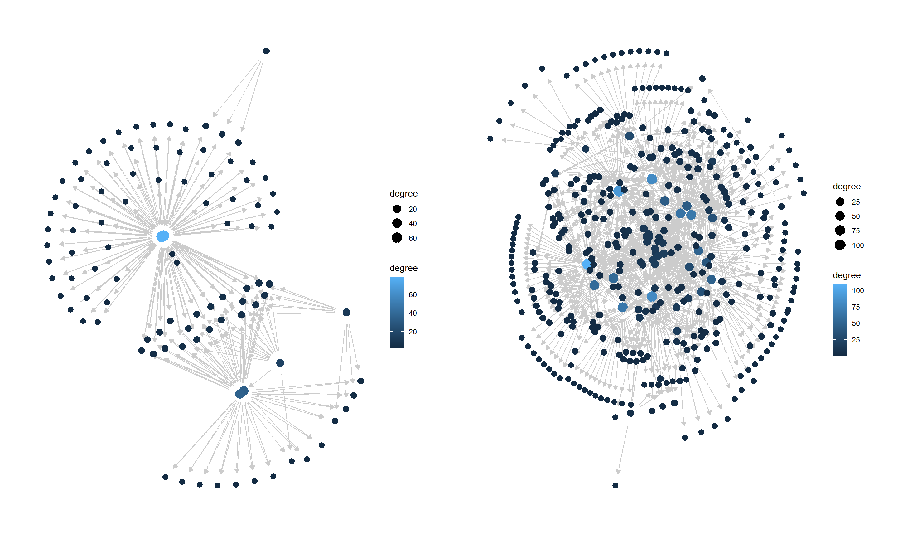
6.4.2 Inference and evaluation
Load the expression data, and bootstrapped network is obtained using GES algorithm. The expression is coarse-grained beforehand. The performance metrics is calculated based on the functions in scstruc.
## DS1
df <- read.csv("De-noised_100G_9T_300cPerT_4_DS1/simulated_noNoise_0.csv", row.names=1)
dim(df)
#> [1]  100 2700
row.names(df) <- paste0("G",row.names(df))
df <- scstruc::superCellMat(as.matrix(df), pca=FALSE)
#>   SuperCell dimension: 100 270
input <- data.frame(t(as.matrix(df)))
ges.res <- pcalg.boot(input, R=25)

calc.auprc(ref.bn.ds1, ges.res)
#> # A tibble: 1 × 3
#>   .metric .estimator .estimate
#>   <chr>   <chr>          <dbl>
#> 1 pr_auc  binary        0.0728
prc.plot(ref.bn.ds1, list("GES"=ges.res))+
    cowplot::theme_cowplot()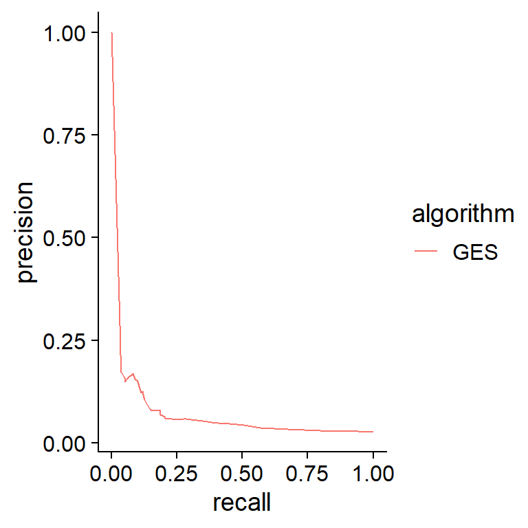
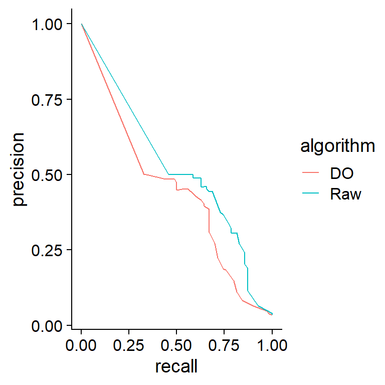
6.5 Adding dropout to GBN
As another method to reproduce dropout in non-SCT data, the add.dropout function is provided. In this example, the function was applied to data sampled from a Gaussian Bayesian network, and the estimation accuracy was compared using the same inference methods.
net <- readRDS("ecoli70.rds")

dat <- rbn(net, 100)
dat2 <- dat * add.dropout(dat, q=0.2)

raw <- pcalg.boot(dat, R=25)
raw.2 <- pcalg.boot(dat2, R=25)

prc.plot(bn.net(net),
    list("Raw"=raw, "DO"=raw.2))+
    cowplot::theme_cowplot()