Chapter 6 The other options

6.1 Using microbiome-related data

library(MicrobiomeProfiler)
data(Rat_data)
ko.res <- enrichKO(Rat_data)
exp.dat <- matrix(abs(rnorm(910)), 91, 10) %>% magrittr::set_rownames(value=Rat_data) %>% magrittr::set_colnames(value=paste0('S', seq_len(ncol(.))))
exp.dat %>% head

FALSE               S1        S2        S3        S4         S5         S6        S7         S8        S9       S10
FALSE K01809 1.0258585 0.5548567 0.4003436 0.6788078 1.13371970 1.41151243 1.8440381 0.97353206 0.5043282 0.2380309
FALSE K00688 0.7298670 0.6963865 1.5619467 0.9205528 0.58716102 0.68760125 0.6945185 0.44622843 1.6735640 1.2809780
FALSE K03388 1.1478900 0.9874183 1.0948022 1.0291543 1.29837354 0.06679942 0.5559601 1.52744298 0.9055871 0.5562262
FALSE K01632 0.7745596 1.3905860 0.8923063 0.3546186 0.52034390 0.60359780 0.3164442 0.06439157 0.3197770 1.1025949
FALSE K07406 0.1379650 0.3549818 1.4843694 0.4554946 0.01794059 2.26569784 0.7371879 1.14979456 1.7924435 0.5045444
FALSE K02991 1.3290375 3.0380460 0.5802602 1.4522863 0.79960704 0.33474238 1.6461427 0.06828655 1.0537423 0.4053420

library(CBNplot)
bngeneplot(ko.res, exp=exp.dat, pathNum=1, orgDb=NULL)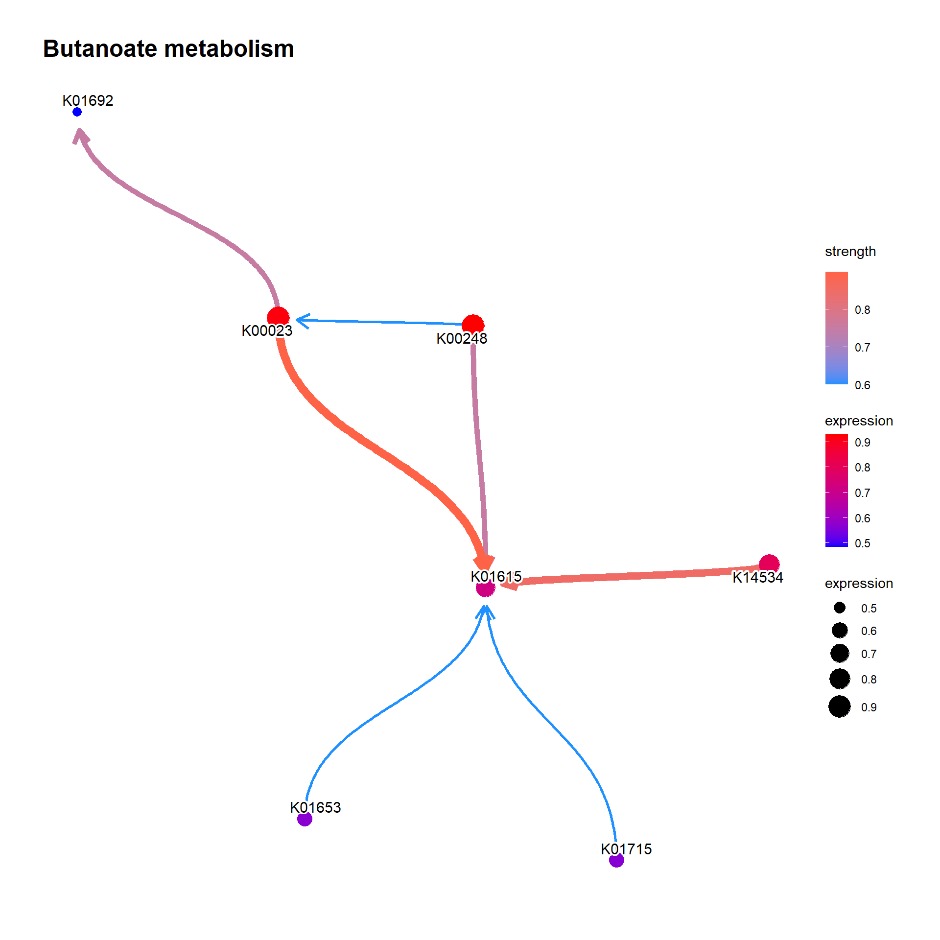

6.2 Discretization

If passed an option disc=TRUE, the continuous variables are discretized using arules::discretize function (Hahsler et al. 2011). The discretization of the gene expression data is discussed in Gallo et al. (2016). If the same discretization is to be applied on the other data like the training and test dataset, you can pass the training samples to tr option, and if some variables are not intended to be discretized, you should pass the column name to remainCont.

bngeneplot(results = pway, exp = vsted, pathNum = 1, disc=TRUE, layout="sugiyama")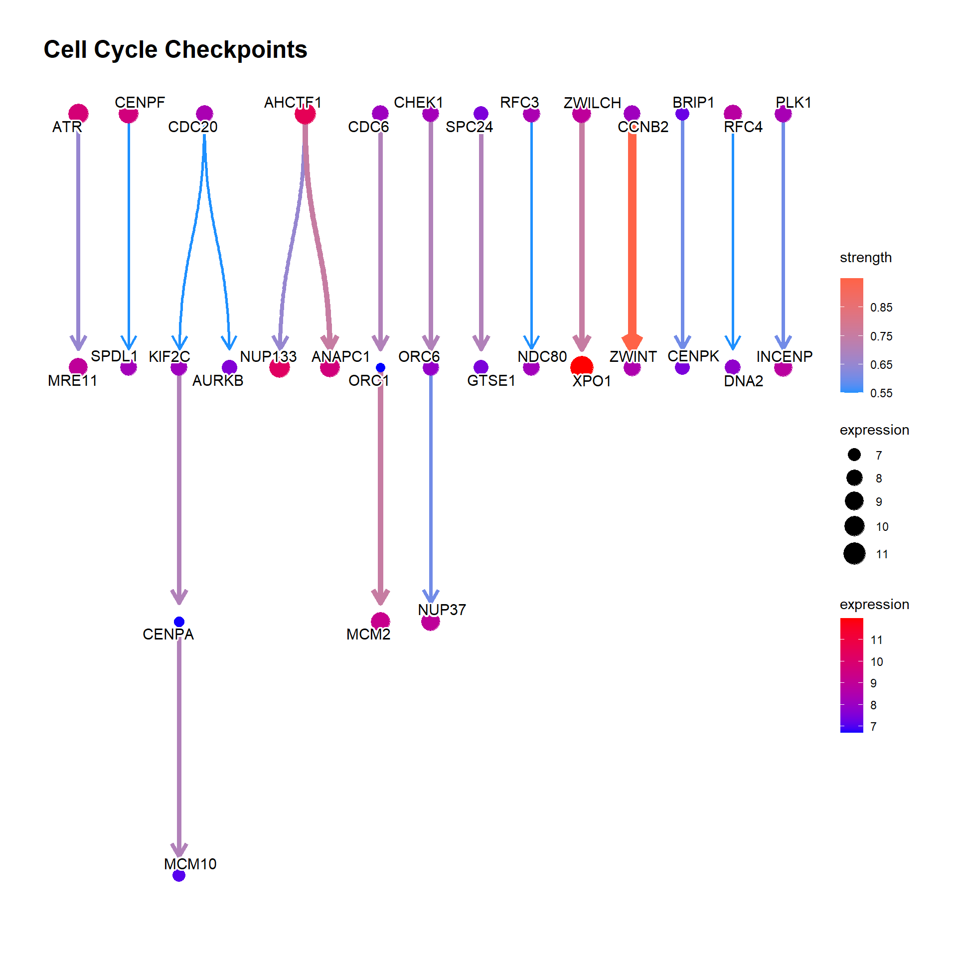

6.3 Custom visualization

6.3.1 The glowing nodes and edges

In addition to the normal plot, custom function of visualization is implemented (bngeneplotCustom and bnpathplotCustom). For example, to effectively visualize the hub genes and edges with high strength by glowing the respective nodes and edges, below is an example using an idea of ggCyberPunk. Additionally, the edge and node colors are fully customizable.

cl = parallel::makeCluster(6)
bngeneplotCustom(results = pway,
                exp = vsted,
                expSample = incSample,
                R=50, cl=cl, layout="nicely", fontFamily="sans",
                pathNum = c(4), strType="normal", sizeDep=TRUE, dep=dep,
                showDir=FALSE, hub=5, glowEdgeNum=5,
                strThresh=0.6, strengthPlot = TRUE)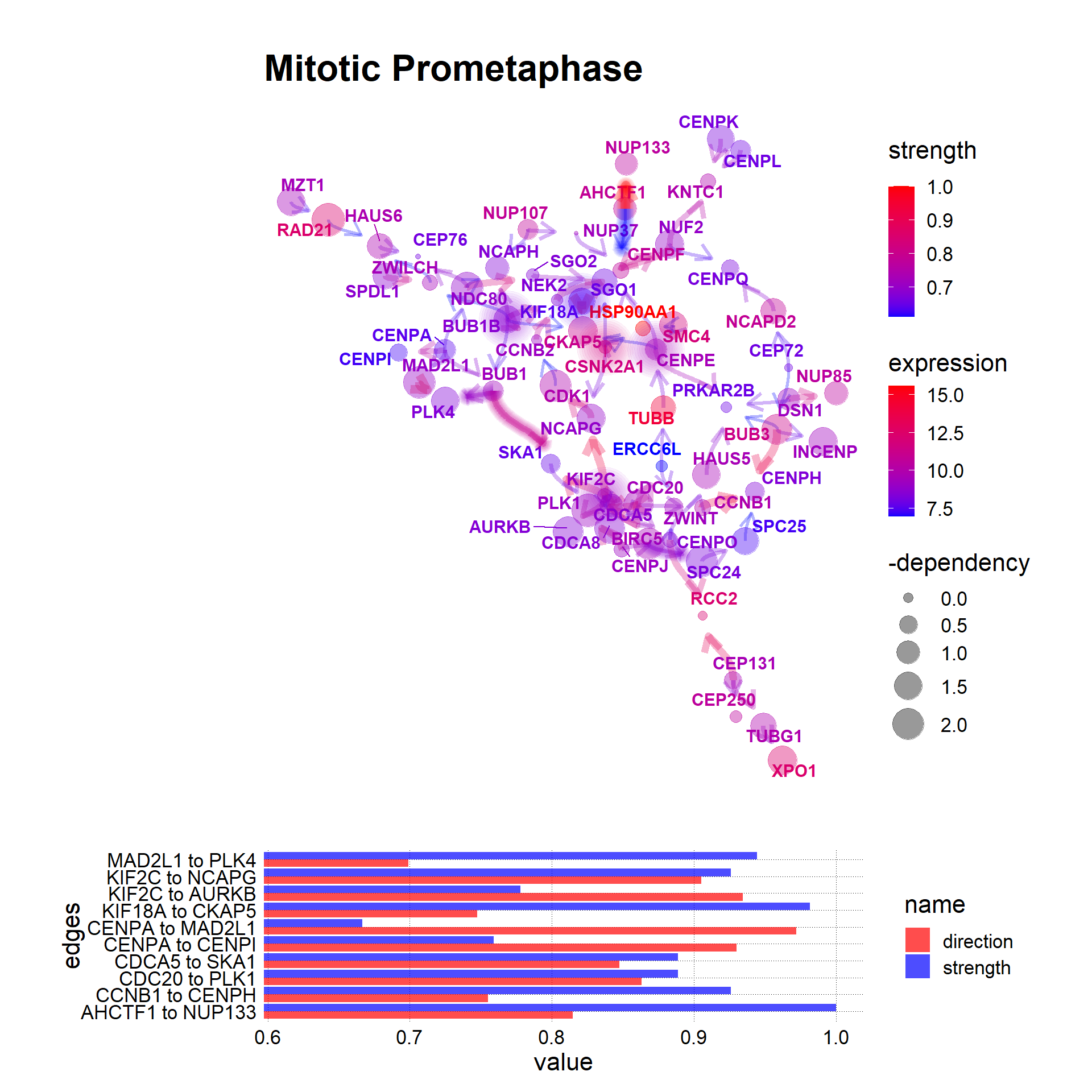

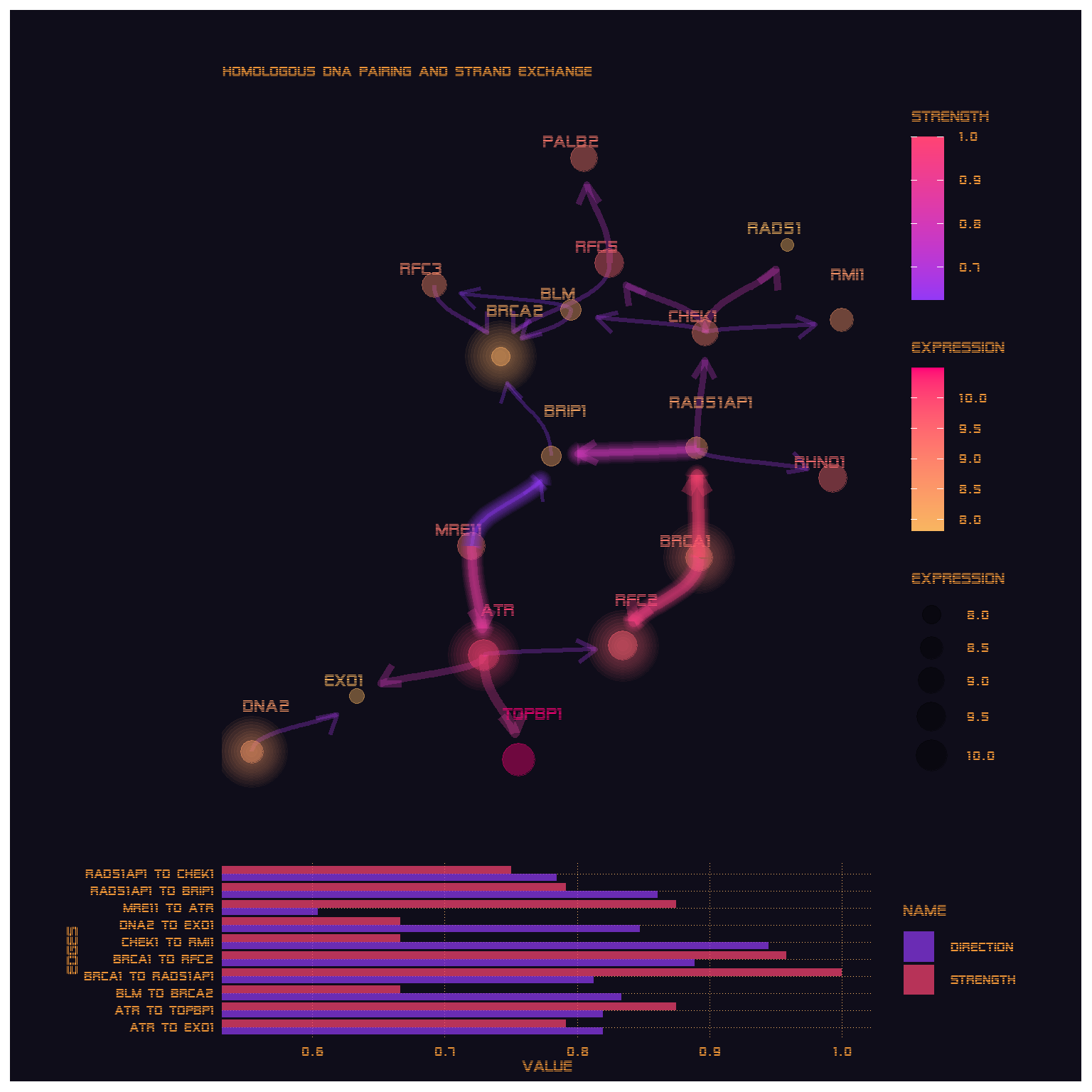
For the demonstrative purpose, using the palettes and fonts of vapoRwave and showtext, the other visualizations are possible. Note that in custom visualization, only the network plot and strength barplot are supported.

## Use alien encounter fonts (http://www.hipsthetic.com/alien-encounters-free-80s-font-family/)
sysfonts::font_add(family="alien",regular="SFAlienEncounters.ttf")
showtext::showtext_auto()
cl = parallel::makeCluster(6)
bngeneplotCustom(results = pway,
                        exp = vsted,
                        expSample = incSample,
                        R=20, cl=cl, fontFamily="alien", labelSize=6,
                        pathNum = c(15), strType="normal",
                        showDir=F, hub=5, glowEdgeNum=5, strThresh=0.6,
                        strengthPlot = T, sizeDep=F, dep=dep, layout="kk",
                        edgePal=c("#9239F6","#FF4373"),
                        nodePal=c("#F8B660","#FF0076"),
                        barLegendKeyCol="#0F0D1A",
                        textCol="#EE9537", titleCol="#EE9537",
                        backCol="#0F0D1A",
                        barAxisCol="#EE9537",
                        barTextCol="#EE9537",
                        barPal=c("#9239F6", "#FF4373"),
                        barPanelGridCol="#FFB967",
                        barBackCol="#0F0D1A",
                        titleSize=14
                        )

parallel::stopCluster(cl)

6.4 Comparing multi scale and standard bootstrapping

cl <- parallel::makeCluster(6)
comparePlot <- bngeneplot(results = pway,
                          exp = vsted, cl=cl, strType="normal",
                          pathNum = 15, R = 50, returnNet=T,
                          shadowText = TRUE)
comparePlotMS <- bngeneplot(results = pway,
                          exp = vsted, cl=cl, strType="ms",
                          pathNum = 15, R = 50, returnNet=T,
                          shadowText = TRUE)

kable(comparePlot$str %>%
    filter(direction>0.5) %>%
    arrange(desc(strength)) %>%
    head())

from	to	strength	direction
TOPBP1	ATR	0.9814815	0.8657407
BRCA1	RAD51AP1	0.9629630	0.5243056
ATR	RFC2	0.9444444	0.5648148
RFC5	XRCC3	0.9074074	0.5160384
CHEK1	RAD51	0.8518519	0.8022487
RAD51AP1	CHEK1	0.8333333	0.7468585

kable(comparePlotMS$str %>%
    filter(direction>0.5) %>%
    arrange(desc(strength)) %>%
    head())

from	to	strength	direction
BRCA1	RAD51AP1	0.9974312	0.5885859
RFC2	ATR	0.9968008	0.6932430
BRIP1	BRCA2	0.9922096	0.7125908
DNA2	BLM	0.9903698	0.5422446
BLM	DNA2	0.9903698	0.8090673
TOPBP1	RMI1	0.9892198	0.5154026

References

Gallo, Cristian A, Rocio L Cecchini, Jessica A Carballido, Sandra Micheletto, and Ignacio Ponzoni. 2016. “Discretization of Gene Expression Data Revised.” Brief. Bioinform. 17 (5): 758–70.

Hahsler, Michael, Sudheer Chelluboina, Kurt Hornik, and Christian Buchta. 2011. “The Arules R-Package Ecosystem: Analyzing Interesting Patterns from Large Transaction Data Sets.” J. Mach. Learn. Res. 12 (57): 2021–25.