Chapter 5 Including clinical variables

5.1 Preparation of data

One of the important reasons of the Bayesian network analysis is assessing the relationship between gene expressions and clinical variables. CBNplot offers incorporating metadata into inference. As a demonstrative purpose, the enrichment analysis results from GSE133624 is applied on data from The Cancer Genome Atlas Program (TCGA) (Cancer Genome Atlas Research Network et al. 2013). Specifically, TCGA-BLCA data is downloaded by the useful library TCGAbiolinks (Colaprico et al. 2016).

library(TCGAbiolinks)
## Load dataset
load(file="tcgablcaData.rda")

We filtered the metadata based on the variables to be included in the inference. In this analysis, age_at_diagnosis and paper_Combined T and LN category, which is a sum of Tumor stage T 1/2 (0) vs. 3/4 (1) and LN negative (0) vs positive (1), are included. We again applied VST on the data.

5.2 Inference of pathway relationship including clinical variables

We assess the relationship between the curated biological pathway information and clinical variables mentioned above. Variables other than expression data can be specified with otherVar, as well as otherVarName for their name. The order of otherVar must be same as column order of expression data. We use all the significant pathways of corrected p-values below 0.05.

bnCov <- bnpathplot(pway,
                    vstedTCGA,
                    nCategory = 1000,
                    adjpCutOff = 0.01,
                    expSample=rownames(metadata),
                    algo="hc", strType="normal",
                    otherVar=metadata,
                    otherVarName=c("Age", "Category"),
                    R=50, cl=parallel::makeCluster(10),
                    returnNet=T,
                    shadowText=T)
## Check DAG
igraph::is.dag(as.igraph(bnCov$av))

FALSE [1] TRUE

## Fit the parameter to network based on the data
bnFit <- bn.fit(bnCov$av, bnCov$df)

Plot the resulting network.

bnCov$plot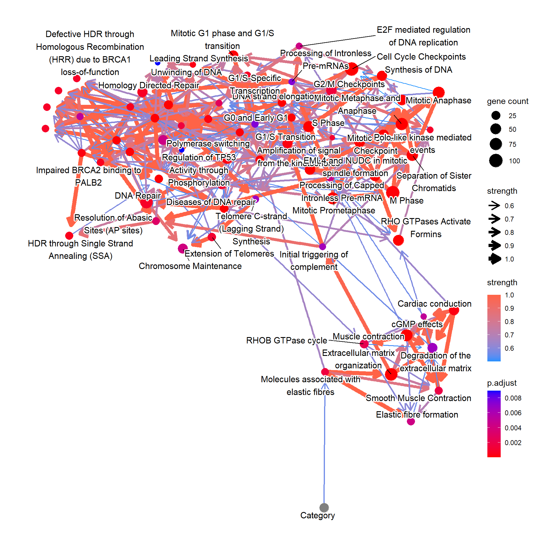

5.3 Conditional probability query

Next we perform conditional probability queries by the bnlearn function cpdist to elucidate how the clinical variables affect pathway regulation. First we fit the inferred network to the original data. These are stored in the named list. Logic sampling is performed unless otherwise stated.

Perform cpdist, and visualize the distribution of “Molecules associated with elastic fibres” conditional on the tumor category using ggdist.

library(bnlearn)
library(ggdist)
library(ggplot2)

candPath <- "Molecules associated with elastic fibres"

efz <- cpdist(bnFit, nodes=c(candPath), evidence=(Category==0))
efo <- cpdist(bnFit, nodes=c(candPath), evidence=(Category==1))
eft <- cpdist(bnFit, nodes=c(candPath), evidence=(Category==2))

effect = data.frame(
  val = c(efz[,1], efo[,1], eft[,1]),
  stage = c(rep("0",nrow(efz)), rep("1", nrow(efo)), rep("2", nrow(eft)))
)

disMean <- effect %>% group_by(stage) %>% summarise(mean=mean(val))
stageWMean <- paste0(disMean$stage, " (mean=", round(disMean$mean,3), ")")
effect$stageLabel <- c(rep(stageWMean[1],nrow(efz)), rep(stageWMean[2], nrow(efo)), rep(stageWMean[3], nrow(eft)))

ggplot(effect, aes(x=val, y=stage, color=stageLabel, fill=stageLabel)) +
    scale_color_manual(values=c("steelblue","gold","tomato")) +
    scale_fill_manual(values=c("steelblue","gold","tomato")) +
    stat_dotsinterval() + theme_bw() + ggtitle(candPath)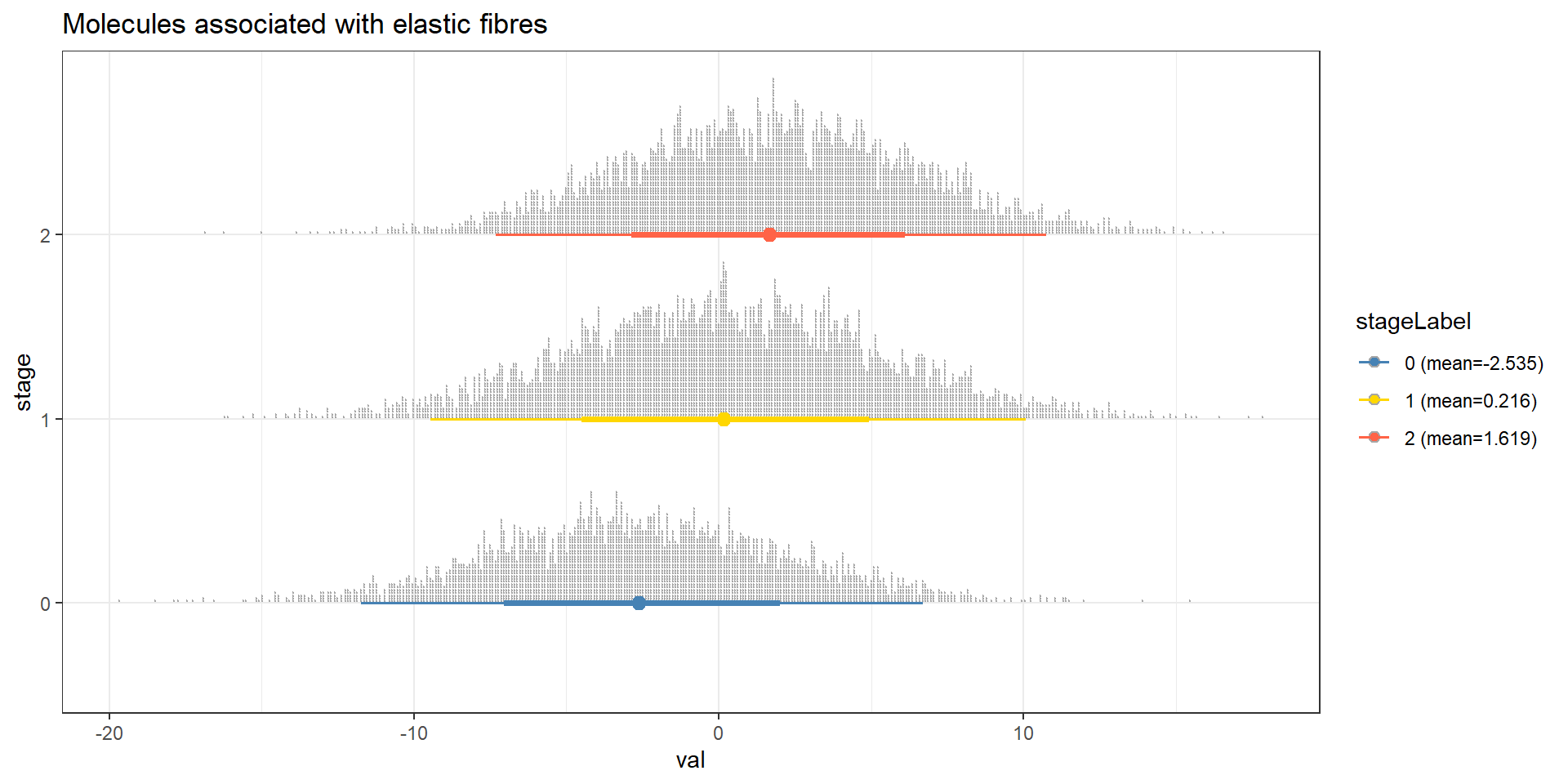

How the down-regulation in “Cell Cycle Checkpoints” affects the other pathways? This time using the importance sampling method, likelihood weighting.

predNodes <- names(bnFit)
predNodes <- predNodes[predNodes != "Cell Cycle Checkpoints"]
maxVal <- max(bnCov$df[candPath])
minVal <- min(bnCov$df[candPath])

lowCCC <- cpdist(bnFit, nodes=predNodes, evidence=list("Cell Cycle Checkpoints"=minVal), method="lw")
lowW <- attributes(lowCCC)$weights
highCCC <- cpdist(bnFit, nodes=predNodes, evidence=list("Cell Cycle Checkpoints"=maxVal), method="lw")
highW <- attributes(highCCC)$weights

## Remove the factor
highCCC$Category <- NULL
lowCCC$Category <- NULL

difMeanCCC <- apply(highCCC, 2, function(x) weighted.mean(x, highW)) - apply(lowCCC, 2, function(x) weighted.mean(x, lowW))

## Top absolute value
kable(head(difMeanCCC[order(abs(difMeanCCC), decreasing=TRUE)]), col.names=c("difference"))

	difference
M Phase	23.15520
Mitotic Prometaphase	20.93115
Mitotic Metaphase and Anaphase	20.70000
Mitotic Anaphase	20.56985
Separation of Sister Chromatids	19.35587
Resolution of Sister Chromatid Cohesion	19.16356

## Reflect the difference in the plot modifying ggplot2 object
changeCol <- bnCov$plot$data
difMeanCCC <- difMeanCCC[changeCol$name]
names(difMeanCCC) <- changeCol$name
changeCol$color <- difMeanCCC

## Replace the color, change the legend
bnCov$plot$data <- changeCol
bnCov$plot + scale_color_continuous(low="blue",high="red",name="difference")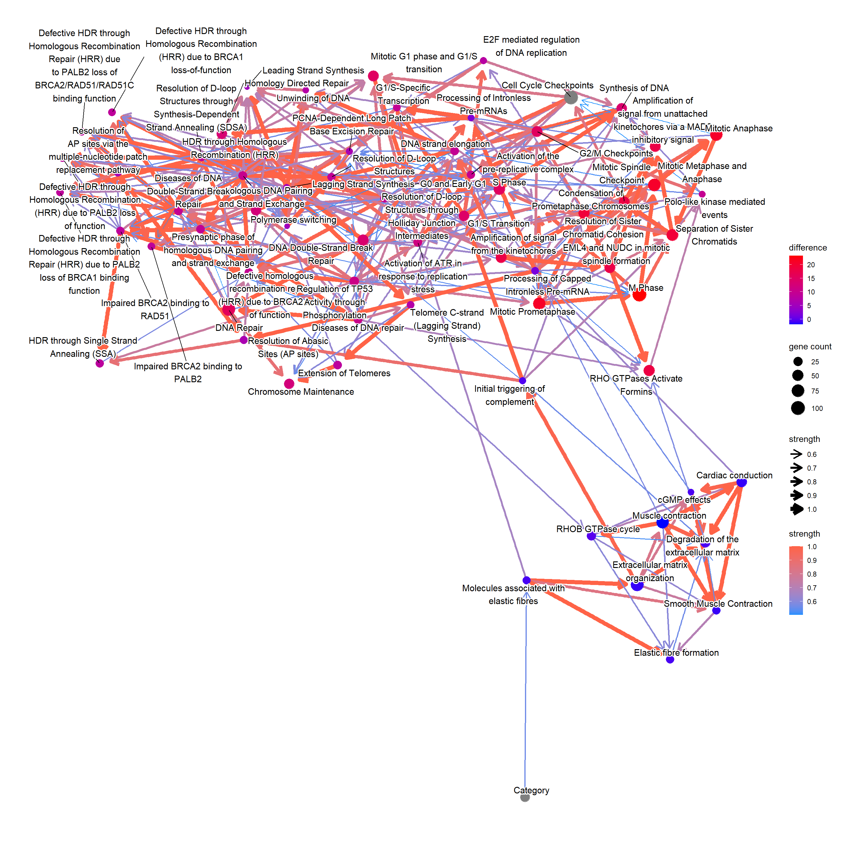

5.4 Gene relationship with variables

For the genes in interesting pathway, clinical variables can be incorporated too. We investigated the genes involved in the reactome “Molecules associated with elastic fibres”.

num <- which(pway@result$Description=="Molecules associated with elastic fibres")
bnGeneCov <- bngeneplot(pway,
                vstedTCGA, pathNum=num,
                expSample=rownames(metadata),
                otherVar=metadata,
                hub=5, R=100,
                otherVarName=c("Age","Category"),
                cl=parallel::makeCluster(10),
                returnNet=T)

Plot the resulting network of genes.

## Plot
bnGeneCov$plot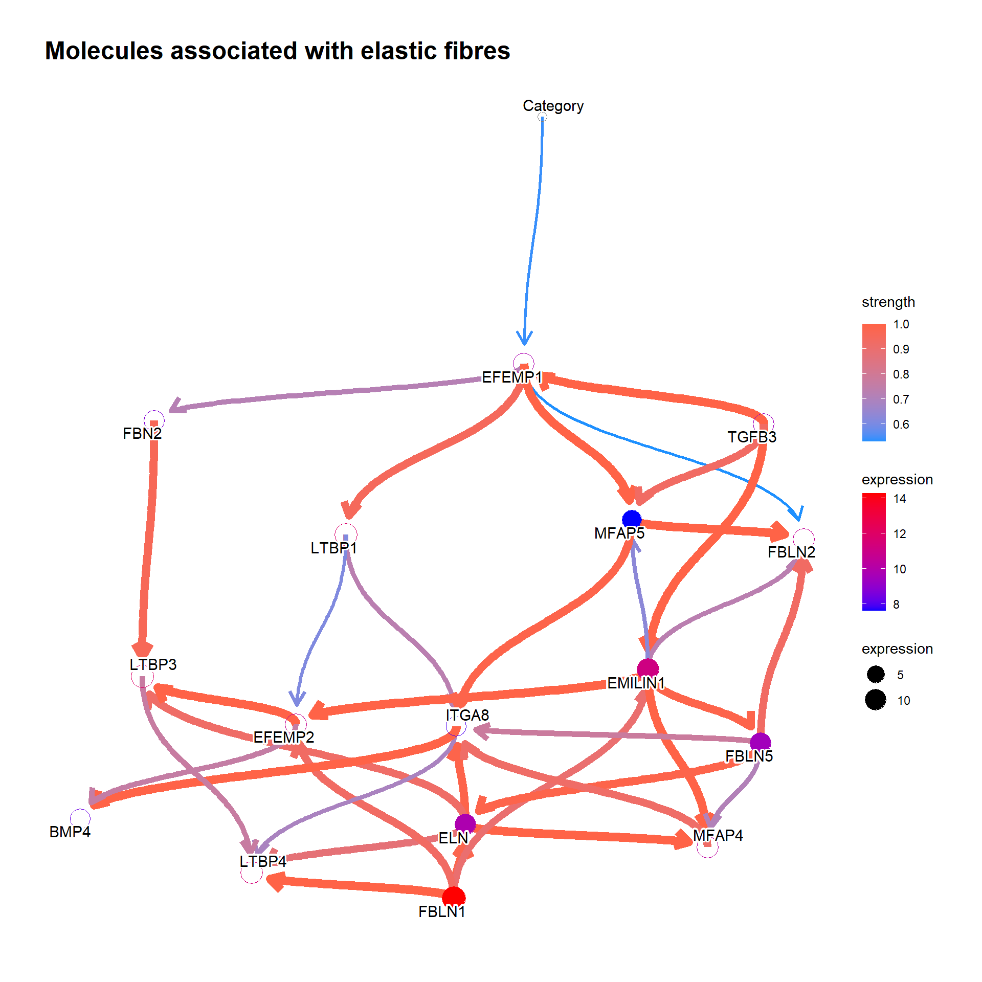

## Check DAG
igraph::is.dag(as.igraph(bnGeneCov$av))

FALSE [1] TRUE

## Fit the parameter to network based on the data
bnFitGene <- bn.fit(bnGeneCov$av, bnGeneCov$df)

Perform cpdist, and examine the mean and distribution using ggdist. We can see that the expression of the gene EFEMP1, which is reported to be a candidate for a biomarker of aggressive bladder cancer or therapeutic targets (Han et al. 2017), is going up with each stage.

candGene <- "EFEMP1"
efz <- cpdist(bnFitGene, nodes=c(candGene), evidence=(Category==0))
efo <- cpdist(bnFitGene, nodes=c(candGene), evidence=(Category==1))
eft <- cpdist(bnFitGene, nodes=c(candGene), evidence=(Category==2))

effect = data.frame(
  val = c(efz[,1], efo[,1], eft[,1]),
  stage = c(rep("0",nrow(efz)), rep("1", nrow(efo)), rep("2", nrow(eft)))
)

disMean <- effect %>% group_by(stage) %>% summarise(mean=mean(val))
stageWMean <- paste0(disMean$stage, " (mean=", round(disMean$mean,3), ")")
effect$stageLabel <- c(rep(stageWMean[1],nrow(efz)), rep(stageWMean[2], nrow(efo)), rep(stageWMean[3], nrow(eft)))

ggplot(effect, aes(x=val, y=stage, color=stageLabel, fill=stageLabel)) +
    scale_color_manual(values=c("steelblue","gold","tomato")) +
    scale_fill_manual(values=c("steelblue","gold","tomato")) +
    stat_dotsinterval() + theme_bw() + ggtitle(candGene)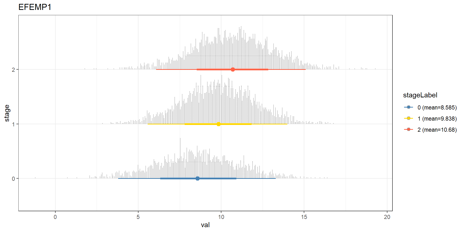

We can reflect the difference to the plot. In the previous EFEMP1 plot:

candGene <- names(bnFitGene)
candGene <- candGene[candGene != "Category"]
efz2 <- cpdist(bnFitGene, nodes=candGene, evidence=(Category==0))
eft2 <- cpdist(bnFitGene, nodes=candGene, evidence=(Category==2))

difMean <- apply(eft2, 2, mean) - apply(efz2, 2, mean)

changeCol <- bnGeneCov$plot$data
difMean <- difMean[changeCol$name]
names(difMean) <- changeCol$name
changeCol$color <- difMean

## Replace shape and color
changeCol$shape <- rep(19, dim(bnGeneCov$plot$data)[1])
bnGeneCov$plot$data <- changeCol
bnGeneCov$plot + scale_color_continuous(low="blue",high="red",name="difference")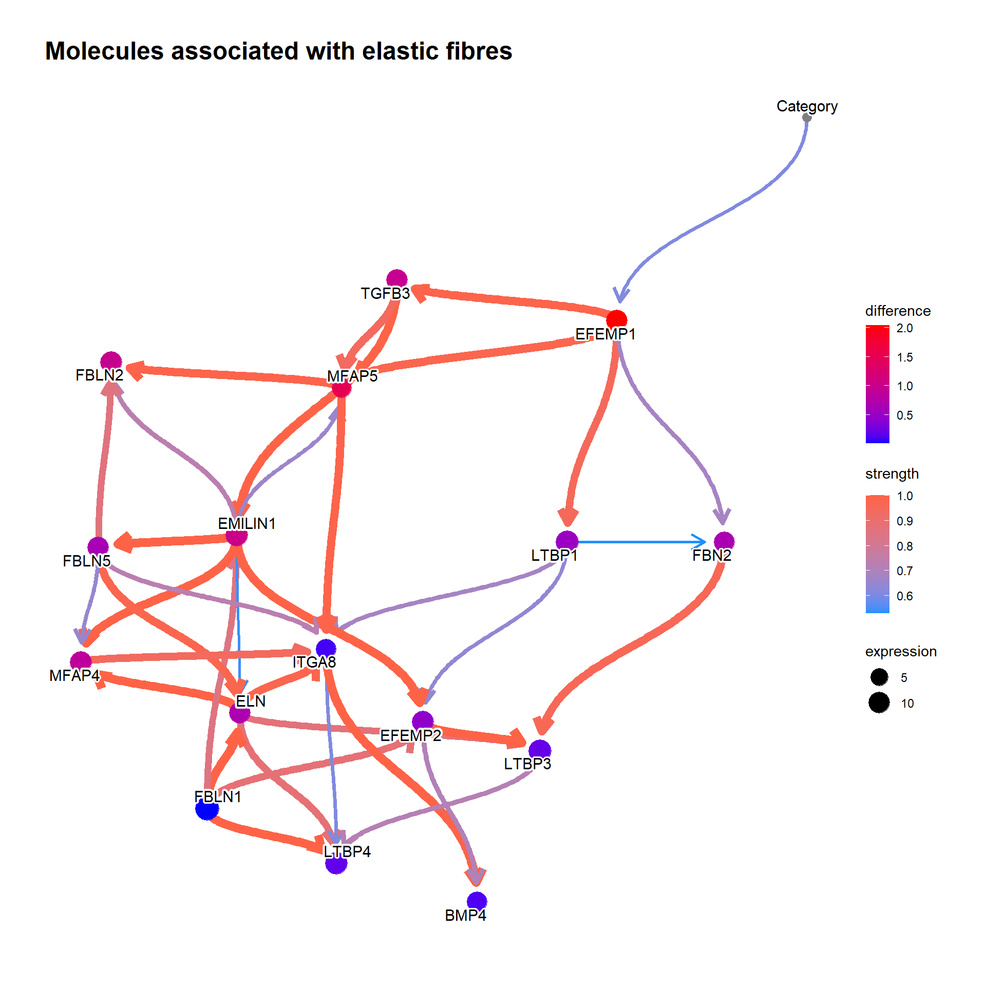

5.5 Confirming the existing knowledge

To confirm the validity of the inferred Bayesian network, we can focus on some genes that is already validated to be related to clinical information or is incorporated into the daily clinical practice. To obtain the pathways that include the specific gene, one can use obtainPath function. This time we focus on the gene MMP2, as the gene has been reported to be related to clinical variables in bladder cancer (Vasala, Pääkkö, and Turpeenniemi-Hujanen 2003; Fouad et al. 2019; Winerdal et al. 2018).

pathSub <- obtainPath(pway, "MMP2")

Using the top pathway involving MMP2, construct the network and plot.

bnGeneCov2 <- bngeneplot(pathSub,
                vstedTCGA, pathNum=1,
                expSample=rownames(metadata),
                otherVar=metadata,
                hub=5, R=100, algo="hc",
                otherVarName=c("Age","Category"),
                cl=parallel::makeCluster(10),
                returnNet=T)

bnGeneCov2$plot

bnGeneCov2Fit <- bn.fit(bnGeneCov2$av, bnGeneCov2$df)

Predict the distribution.

candGene <- "MMP2"

mz <- cpdist(bnGeneCov2Fit, nodes=c(candGene), evidence=(Category==0), method="ls")
mo <- cpdist(bnGeneCov2Fit, nodes=c(candGene), evidence=(Category==1), method="ls")
mt <- cpdist(bnGeneCov2Fit, nodes=c(candGene), evidence=(Category==2), method="ls")

effect = data.frame(
  val = c(mz[,1], mo[,1], mt[,1]),
  stage = c(rep("0",nrow(mz)), rep("1", nrow(mo)), rep("2", nrow(mt)))
)

disMean <- effect %>% group_by(stage) %>% summarise(mean=mean(val))
stageWMean <- paste0(disMean$stage, " (mean=", round(disMean$mean,3), ")")
effect$stageLabel <- c(rep(stageWMean[1],nrow(mz)), rep(stageWMean[2], nrow(mo)), rep(stageWMean[3], nrow(mt)))

ggplot(effect, aes(x=val, y=stage, color=stageLabel, fill=stageLabel)) +
    scale_color_manual(values=c("steelblue","gold","tomato")) +
    scale_fill_manual(values=c("steelblue","gold","tomato")) +
    stat_dotsinterval() + theme_bw() + ggtitle(candGene)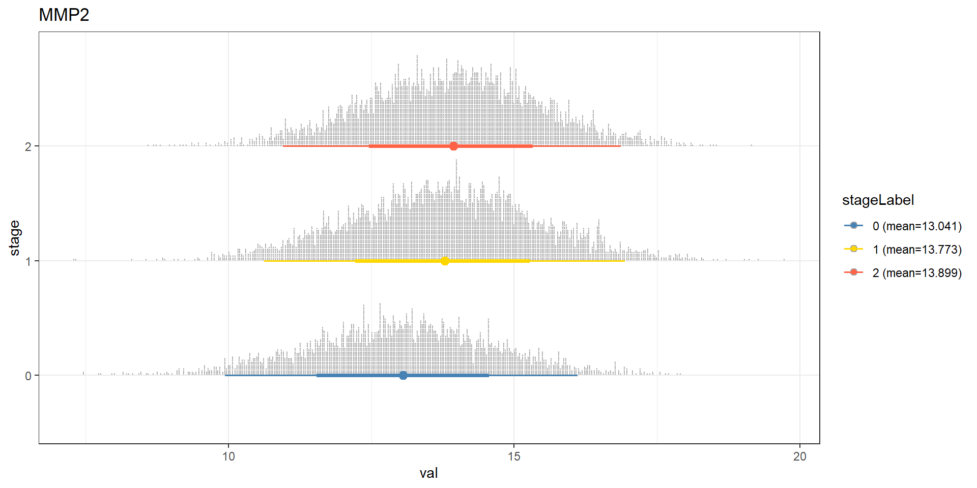

It is interesting to investigate whether the result is similar in the other database, like Gene Ontology doing the same analysis.

## Perform the same analysis on GO enrichment result
pathSubGO <- obtainPath(pwayGO, "MMP2")
pathSubGO@result[1:5, c("Description","geneID","Count")]

FALSE                                   Description
FALSE GO:0001968                fibronectin binding
FALSE GO:0004222      metalloendopeptidase activity
FALSE GO:0008237          metallopeptidase activity
FALSE GO:0004252 serine-type endopeptidase activity
FALSE GO:0008236     serine-type peptidase activity
FALSE                                                                                                                                                                                                                             geneID
FALSE GO:0001968                                                                                                                                           MYOC/FSTL3/FBLN1/MMP2/CCDC80/VEGFA/CCN2/THBS1/SFRP2/EPHA1/IGFBP6/LRRC15/SSC5D
FALSE GO:0004222                                                         NRDC/MMP2/MMP11/ADAM2/COPS5/NLN/MMP19/MMP24/ADAMTS8/MMP27/MMP13/ADAM10/ECE2/ADAM33/ADAM17/ADAMTS1/ADAMTS5/ADAMTS4/MMP10/ADAMTS20/PAPPA/LMLN/MMP23B/MMP1/TRABD2B
FALSE GO:0008237 NAALAD2/NRDC/MMP2/MMP11/CPQ/ADAM2/PSMD14/COPS5/CPXM2/XPNPEP2/NLN/MMP19/STAMBP/MMP24/CPA4/ADAMTS8/MMP27/MMP13/ADAM10/ECE2/ADAM33/ADAM17/ADAMTS1/ADAMTS5/ADAMTS4/MYSM1/CPA3/MMP10/ADAMTS20/PAPPA/LMLN/MMP23B/MMP1/TRABD2B
FALSE GO:0004252                                                                             LTF/MMP2/CMA1/TPSD1/MMP11/ACR/CTSG/GZMH/GZMK/TPSG1/MMP19/PCSK2/F10/MASP1/F12/CTSV/MMP13/C1R/MMP10/KLK6/TPSAB1/C1S/MMP1/TPSB2/GZMM/ELANE/CFD
FALSE GO:0008236                                                                LTF/NAALAD2/MMP2/CMA1/TPSD1/MMP11/ACR/CTSG/GZMH/CPVL/GZMK/TPSG1/MMP19/PCSK2/F10/MASP1/F12/CTSV/MMP13/C1R/MMP10/KLK6/TPSAB1/C1S/MMP1/TPSB2/GZMM/ELANE/CFD
FALSE            Count
FALSE GO:0001968    13
FALSE GO:0004222    25
FALSE GO:0008237    34
FALSE GO:0004252    27
FALSE GO:0008236    29

num <- 1:2
bnCovGO <- bngeneplot(pathSubGO,
                vstedTCGA,
                pathNum=num,
                algo="hc",
                expSample=rownames(metadata),
                otherVar=metadata,
                R=300, layout="sugiyama",
                otherVarName=c("Age","Category"),
                cl=parallel::makeCluster(10),
                returnNet=TRUE)

bnCovGO$av$nodes$Category

FALSE $mb
FALSE [1] "CCDC80"
FALSE 
FALSE $nbr
FALSE [1] "CCDC80"
FALSE 
FALSE $parents
FALSE character(0)
FALSE 
FALSE $children
FALSE [1] "CCDC80"

bnGeneCovGOFit <- bn.fit(bnCovGO$av, bnCovGO$df)

mz <- cpdist(bnGeneCovGOFit, nodes=c(candGene), evidence=(Category==0), method="ls")
mo <- cpdist(bnGeneCovGOFit, nodes=c(candGene), evidence=(Category==1), method="ls")
mt <- cpdist(bnGeneCovGOFit, nodes=c(candGene), evidence=(Category==2), method="ls")

effect = data.frame(
  val = c(mz[,1], mo[,1], mt[,1]),
  stage = c(rep("0",nrow(mz)), rep("1", nrow(mo)), rep("2", nrow(mt)))
)

disMean <- effect %>% group_by(stage) %>% summarise(mean=mean(val))
stageWMean <- paste0(disMean$stage, " (mean=", round(disMean$mean,3), ")")
effect$stageLabel <- c(rep(stageWMean[1],nrow(mz)), rep(stageWMean[2], nrow(mo)), rep(stageWMean[3], nrow(mt)))

ggplot(effect, aes(x=val, y=stage, color=stageLabel, fill=stageLabel)) +
    scale_color_manual(values=c("steelblue","gold","tomato")) +
    scale_fill_manual(values=c("steelblue","gold","tomato")) +
    stat_dotsinterval() + theme_bw() + ggtitle(candGene) + labs(caption=paste(pathSubGO@result$Description[num], collapse="\n"))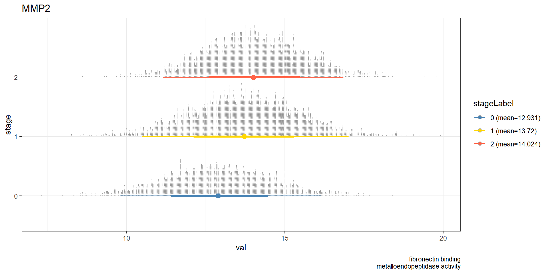

5.6 Investigating the network based on the clinical question

After confirming the knowledge, it is interesting to test how difference in clinical variables affect gene expression. bnlearn can naturally handle this again using cpdist. We now include two more variables, age_at_diagnosis, gender, paper_Noninvasive.bladder.cancer.therapy, paper_Combined.T.and.LN.category. Inference based on these information, we can ask:

Which genes have the biggest expression differences between those treated with BCG and with none, considering the networks of genes and clinical variables of age, gender, tumor category in TCGA-BLCA dataset using genes significantly differed in GSE133624 and involved in curated biological pathways related to MMP2?

## Subset to significant pathways, and those related to MMP2
pway@result <- subset(pway@result, p.adjust<0.05)
pathSub <- obtainPath(pway, "MMP2")

bnCovGene3 <- bngeneplot(pathSub,
                vstedBCG,
                pathNum = seq_len(nrow(pathSub)),
                expSample=rownames(metadata),
                otherVar=metadata,
                hub=5, R=50,
                otherVarName=c("Age","Gender","Therapy","Category"),
                cl=parallel::makeCluster(10),
                returnNet=T)
bnCovGene3Fit <- bn.fit(bnCovGene3$av, bnCovGene3$df)

allGenes <- names(bnCovGene3$av$nodes)
allGenes <- allGenes[!allGenes %in% c("Age","Gender","Therapy","Category")]
no <- cpdist(bnCovGene3Fit, nodes=allGenes, evidence=(Therapy=="none"), method="ls")
bcg <- cpdist(bnCovGene3Fit, nodes=allGenes, evidence=(Therapy=="Bacillus Calmette.Guerin (BCG)"), method="ls")

difMean <- data.frame(apply(bcg, 2, mean)-apply(no, 2, mean))
difMean$name <- rownames(difMean)
colnames(difMean) <- c("difference","name")
difMean <- difMean[order(abs(difMean$difference), decreasing=T),]
kable(head(difMean, n=5))

	difference	name
COL25A1	0.2344216	COL25A1
MFAP5	0.1834830	MFAP5
COL11A1	0.1494830	COL11A1
COL10A1	0.1381034	COL10A1
LAMC2	-0.1340511	LAMC2

5.7 Classification using BN

Inferred BN can be used as a classifier of conditions. In this analysis, we perform the classification of whether the cancer samples are harboring TP53 mutation or not (column paper_mutation in TP53). First, we make a metadata table as same as the above examples.

metadata <- data.frame(tcgaData@colData) %>%
  dplyr::select(age_at_diagnosis, gender, paper_mutation.in.TP53, paper_Combined.T.and.LN.category) %>% na.omit() %>%
  filter(paper_mutation.in.TP53!="ND") %>%
  filter(paper_Combined.T.and.LN.category!="ND")
table(metadata$paper_mutation.in.TP53)

FALSE 
FALSE  no yes 
FALSE 184 163

## Set TP53 status to numeric of 0/1.
metadata$paper_mutation.in.TP53 <- as.numeric(as.factor(metadata$paper_mutation.in.TP53))-1
metadata$age_at_diagnosis <- as.numeric(scale(metadata$age_at_diagnosis))
metadata$paper_Combined.T.and.LN.category <- as.factor(metadata$paper_Combined.T.and.LN.category)
metadata$gender <- as.factor(metadata$gender)

Split the data to train/test according to TP53 mutation status using caret (Kuhn 2008). In this analysis, the five-fold cross validation (stratified) is performed. Fit the model using the expression of genes in the pathway. This time the classification performance of significant pathways (corrected p < 1e-5) are to be compared. onlyDf option can be enabled to return only the data.frame containing data for prediction, useful for testing purpose, and using the resulting data for the other softwares.

set.seed(53) # Seed for split
trainIndex <- caret::createFolds(factor(metadata$paper_mutation.in.TP53), k = 5, list = TRUE, returnTrain=TRUE)
allnets <- list() ## Store network in the list
allClassRes <- list() ## Store prediction in the list

## Already VSTed DF
load("trainDf.rda")
load("testDf.rda")

for (f in seq_len(5)) {
  nets <- list()
  classRes <- list()
  foldTrainIndex <- trainIndex[[f]]
  ## Recursively fit and test for significant pathways
  for (pnum in seq(1, dim(subset(pway@result, p.adjust<1e-5))[1], 1)) {
      cl <- parallel::makeCluster(12)
      bnCovTrain <- bngeneplot(pway, assay(trainDf[[f]]), pathNum=pnum, layout="sugiyama",
                               expSample=rownames(metadata[foldTrainIndex,]), algo="hc", strType="normal",
                               otherVar=metadata[foldTrainIndex,], otherVarName=c("Age","Gender","TP53","Category"),
                               R=50, cl=cl, returnNet=T)
      ## Return only DF for testing
      bnCovTest <- bngeneplot(pway, assay(testDf[[f]]), pathNum=pnum,
                               expSample=rownames(metadata[-foldTrainIndex,]),
                               otherVar=metadata[-foldTrainIndex,],  otherVarName=c("Age","Gender","TP53","Category"),
                               onlyDf=T)
      
      ## If DAG and TP53 have parents
      if ( igraph::is.dag(bnlearn::as.igraph(bnCovTrain$av)) && length(bnCovTrain$av$nodes$TP53$parents) >= 1 ){
        bnCovLargeFit <- bnlearn::bn.fit(bnCovTrain$av, bnCovTrain$df)
        pred <- sigmoid::sigmoid(predict(bnCovLargeFit, node="TP53", data=bnCovTest, method = "bayes-lw")) # Use sigmoid function
        classRes[[pway@result$Description[pnum]]] <- pred
        nets[[pway@result$Description[pnum]]] <- bnCovTrain
      } else {
        message(paste0("Among pathway ", pway@result$Description[pnum], ", no parent node of TP53 is found, or inferred network is not dag."))
      }
      parallel::stopCluster(cl)    
  }
  allnets[[f]] <- nets
  allClassRes[[f]] <- classRes
}

Using the library pROC, calculate the area under ROC (auROC) (Robin et al. 2011).

library(pROC)
library(ggplotify)

rocDf <- c()
allRocList <- list()
for (f in seq_len(5)) {
  correct <- metadata[-trainIndex[[f]],]$paper_mutation.in.TP53
  predDf <- data.frame(allClassRes[[f]])
  predDf$label <- correct
  
  rocList <- list()
  for (i in seq_len(dim(predDf)[2]-1)){
    rocList[[names(predDf)[i]]] <- roc(predDf$label, predDf[,i], ci=TRUE, direction="<") # check direction
  }
  tmpRocDf <- data.frame(t(data.frame(purrr::map(rocList, function(x) as.numeric(x$auc)))))
  colnames(tmpRocDf) <- c(paste0("auc",f))
  tmpRocDf$name <- rownames(tmpRocDf)
  allRocList[[f]] <- tmpRocDf
}

allRocListDf <- allRocList %>%
  purrr::reduce(left_join, by = "name")

rocMean <- allRocListDf %>%
  rowwise() %>%
  mutate(Min = min(c_across(starts_with("auc")), na.rm=T),
         Max = max(c_across(starts_with("auc")), na.rm=T),
         Mean = mean(c_across(starts_with("auc")), na.rm=T),
         Sd = sd(c_across(starts_with("auc")), na.rm=T)) %>%
  select(name ,Mean, Sd) %>%
  arrange(desc(Mean))

kable(rocMean, row.names=FALSE, booktab=TRUE) %>%
  kable_styling(font_size = 10)

name	Mean	Sd
DNA.strand.elongation	0.7586171	0.0476902
S.Phase	0.7442158	0.0417892
RHO.GTPases.Activate.Formins	0.7361936	0.0372955
Activation.of.ATR.in.response.to.replication.stress	0.7313293	0.0309443
Amplification..of.signal.from.unattached..kinetochores.via.a.MAD2..inhibitory.signal	0.7298620	0.0356467
Resolution.of.Sister.Chromatid.Cohesion	0.7245308	0.0627438
Homologous.DNA.Pairing.and.Strand.Exchange	0.7236192	0.0361203
HDR.through.Homologous.Recombination..HRR.	0.7108159	0.0408204
EML4.and.NUDC.in.mitotic.spindle.formation	0.6847067	0.0969711
Mitotic.Spindle.Checkpoint	0.6727978	0.0843631
Separation.of.Sister.Chromatids	0.5731690	0.1567807

Show the resulting network with the top auROC, and the ROC plot using pROC (Robin et al. 2011).

topPath <- rocMean[1,"name"]
candFold <- as.numeric(allRocListDf %>% filter(name == as.character(topPath)) %>% summarize(which.max(c_across(starts_with("auc")))))


## With the CI
candRoc <- data.frame(metadata[-trainIndex[[candFold]],]$paper_mutation.in.TP53)
colnames(candRoc) <- c("label")
candRoc$pred <- as.numeric(unlist(allClassRes[[candFold]][gsub("[.]", " ", as.character(topPath))]))

rocobj1 <- plot.roc(candRoc$label, candRoc$pred, print.auc = TRUE, ci=TRUE, col="black", direction="<",
                  main = "Mutation in TP53", percent=TRUE)
ciobj <- ci.se(rocobj1, specificities = seq(0, 100, 5), progress="none") 
plot(ciobj, type = "shape", col = "steelblue")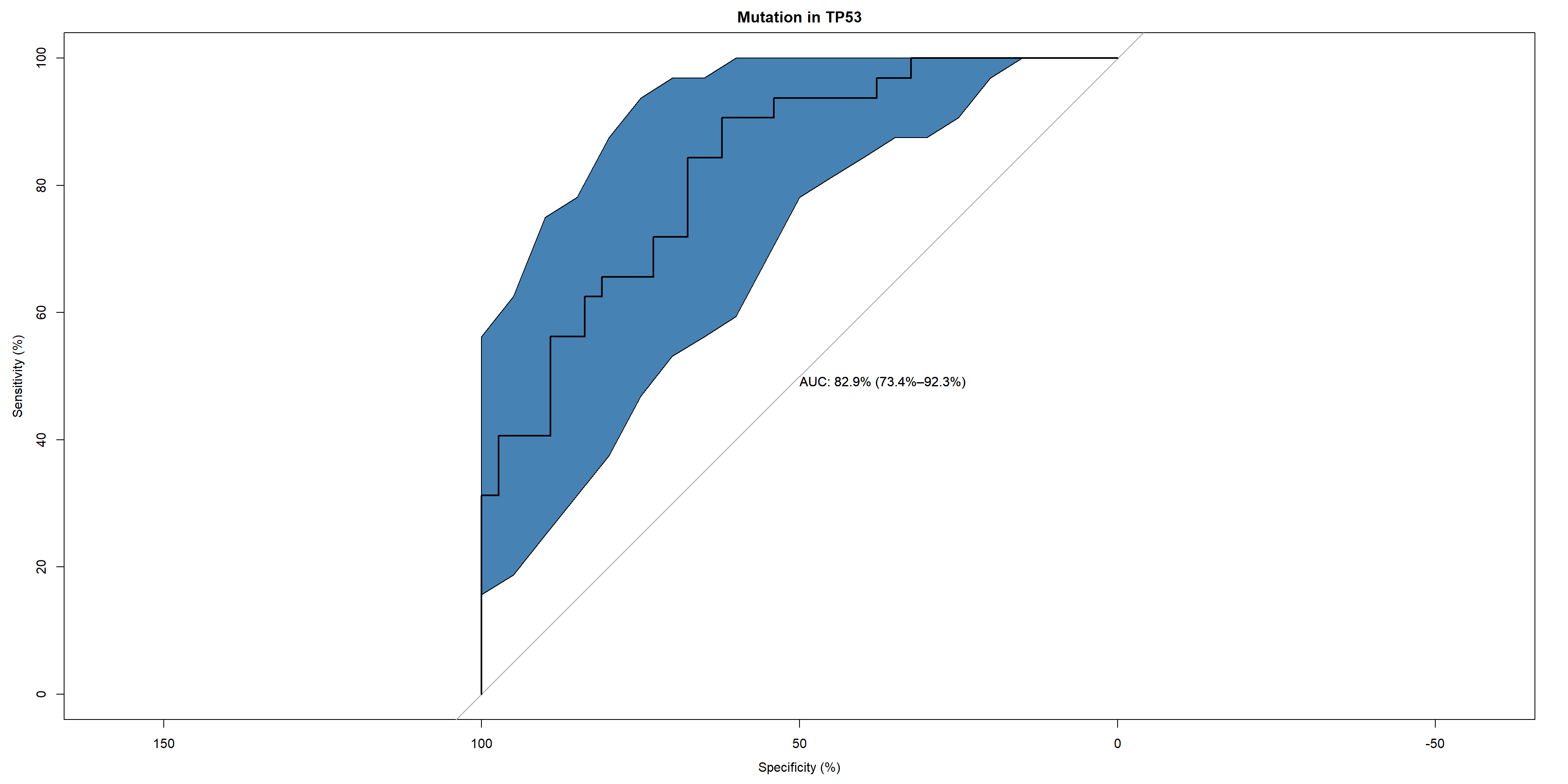

## Along with the network
topNet <- allnets[[candFold]][[gsub("[.]", " ", topPath)]]
topNet$plot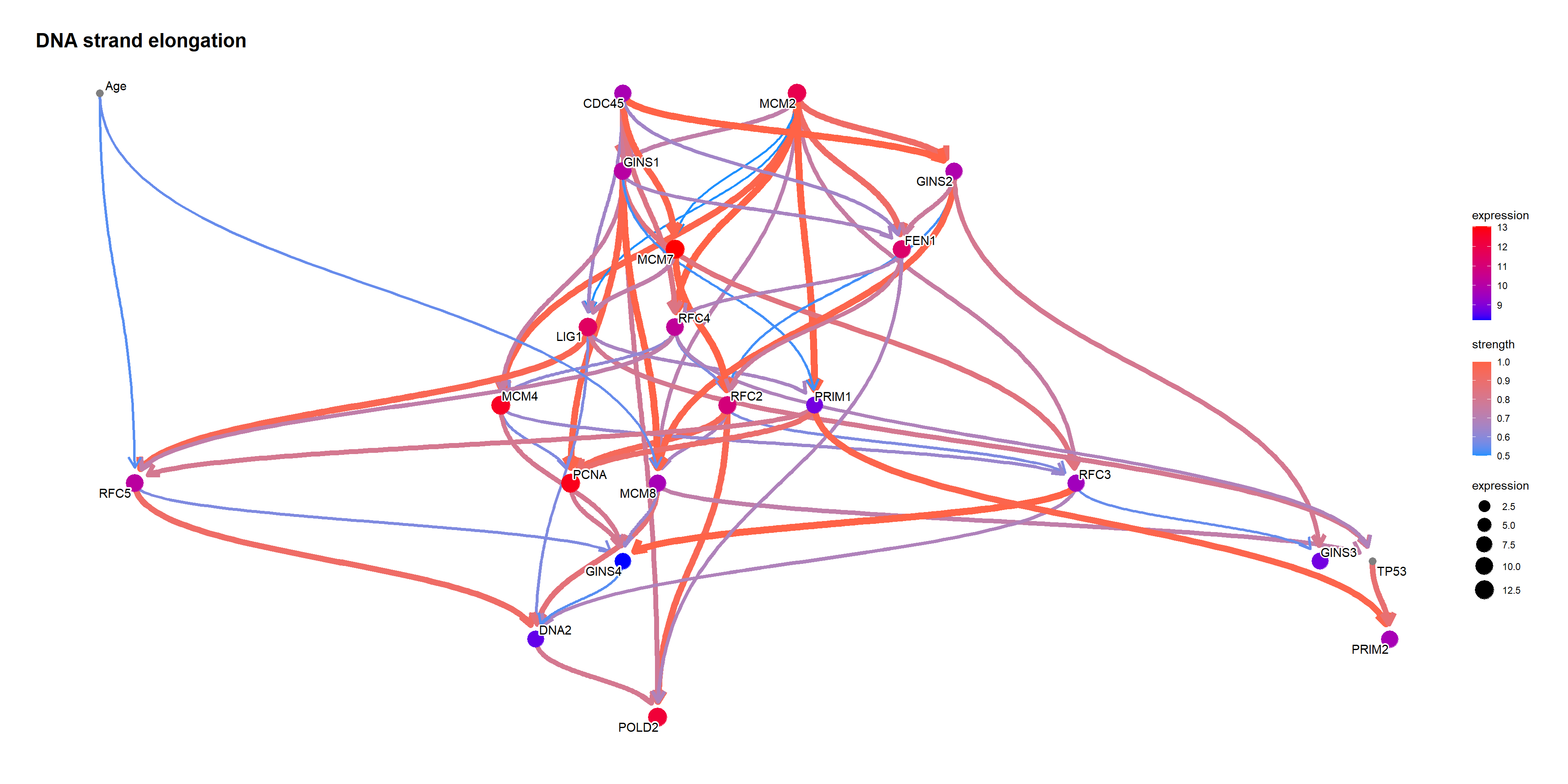

Using bnlearn::cpdist, check the difference in the distribution mean when the value of the node TP53 is above and below 0.5.

topFit <- bnlearn::bn.fit(topNet$av, topNet$df)

candNodes <- names(topNet$av$nodes)
candNodes <- candNodes[!candNodes %in% c("TP53","Category","Gender")]

tp53low <- cpdist(topFit, nodes=candNodes, evidence=(TP53 < 0.5))
dim(tp53low)

FALSE [1] 5225   21

tp53high <- cpdist(topFit, nodes=candNodes, evidence=(TP53 > 0.5))
dim(tp53high)

FALSE [1] 4717   21

difMeanTp53 <- apply(tp53high, 2, mean) - apply(tp53low, 2, mean)
kable(head(difMeanTp53[order(abs(difMeanTp53), decreasing=T)]), col.names=c("difference"))

	difference
MCM2	0.3978904
RFC4	0.3534718
MCM8	0.3250150
PRIM1	0.3243060
PRIM2	0.3031842
GINS4	0.2868035

changeCol <- topNet$plot$data
difMeanTp53 <- difMeanTp53[changeCol$name]
names(difMeanTp53) <- changeCol$name
changeCol$color <- difMeanTp53

## Replace shape and color
topNet$plot$data <- changeCol
topNet$plot + scale_color_continuous(low="blue",high="red",name="difference")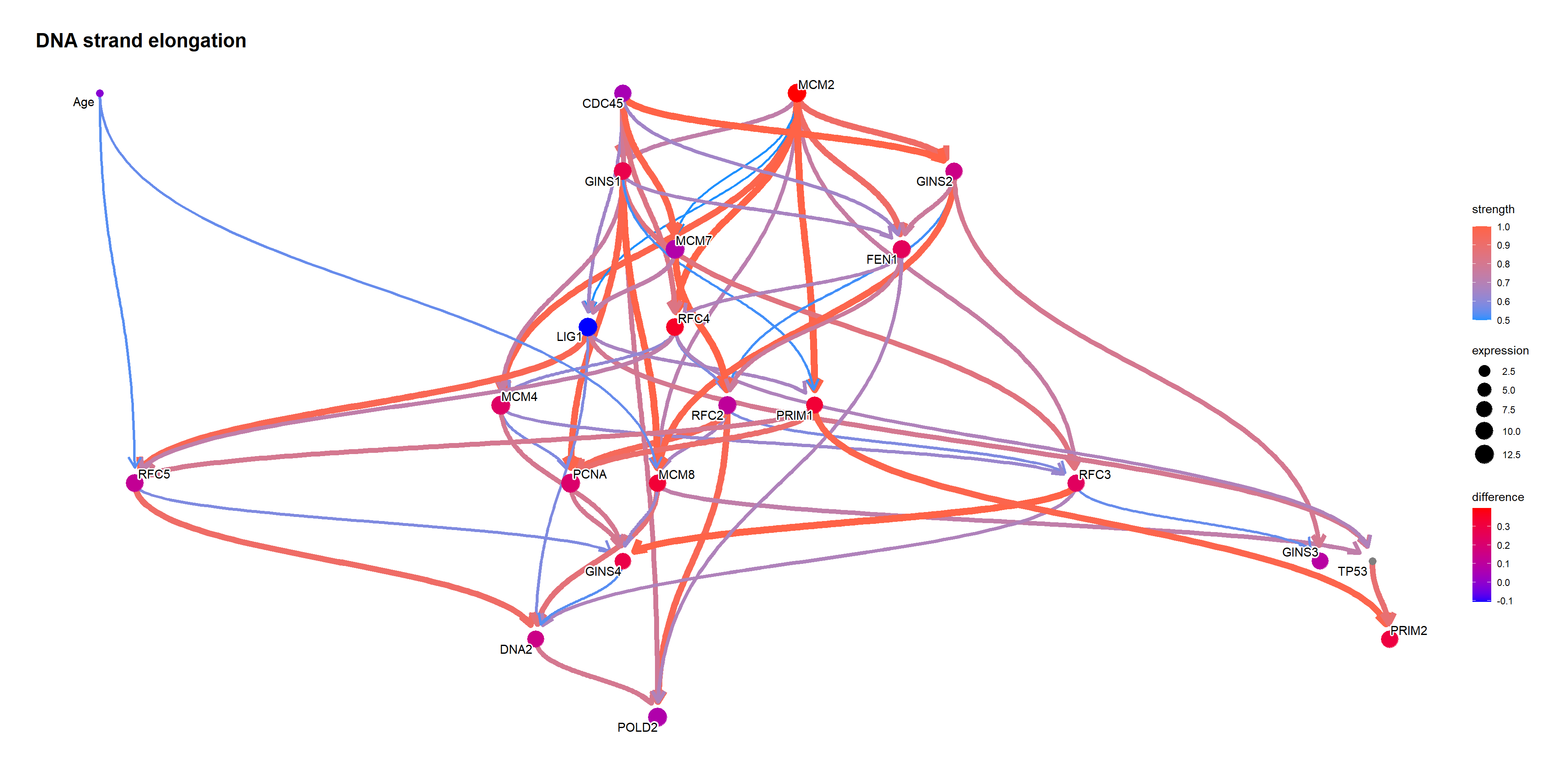

When the TP53 takes the extreme values on logic sampling.

topFit <- bnlearn::bn.fit(topNet$av, topNet$df)

candNodes <- names(topNet$av$nodes)
candNodes <- candNodes[!candNodes %in% c("TP53","Category","Gender")]

tp53low <- cpdist(topFit, nodes=candNodes, evidence=(TP53 < 0.01))
dim(tp53low)

FALSE [1] 1760   21

tp53high <- cpdist(topFit, nodes=candNodes, evidence=(TP53 > 0.99))
dim(tp53high)

FALSE [1] 1552   21

difMeanTp53 <- apply(tp53high, 2, mean) - apply(tp53low, 2, mean)
kable(head(difMeanTp53[order(abs(difMeanTp53), decreasing=T)]), col.names=c("difference"))

	difference
MCM2	0.7375946
RFC4	0.6955627
MCM8	0.5989058
PRIM1	0.5895650
PRIM2	0.5783348
GINS1	0.4874811

changeCol <- topNet$plot$data
difMeanTp53 <- difMeanTp53[changeCol$name]
names(difMeanTp53) <- changeCol$name
changeCol$color <- difMeanTp53

## Replace shape and color
topNet$plot$data <- changeCol
topNet$plot + scale_color_continuous(low="blue",high="red",name="difference")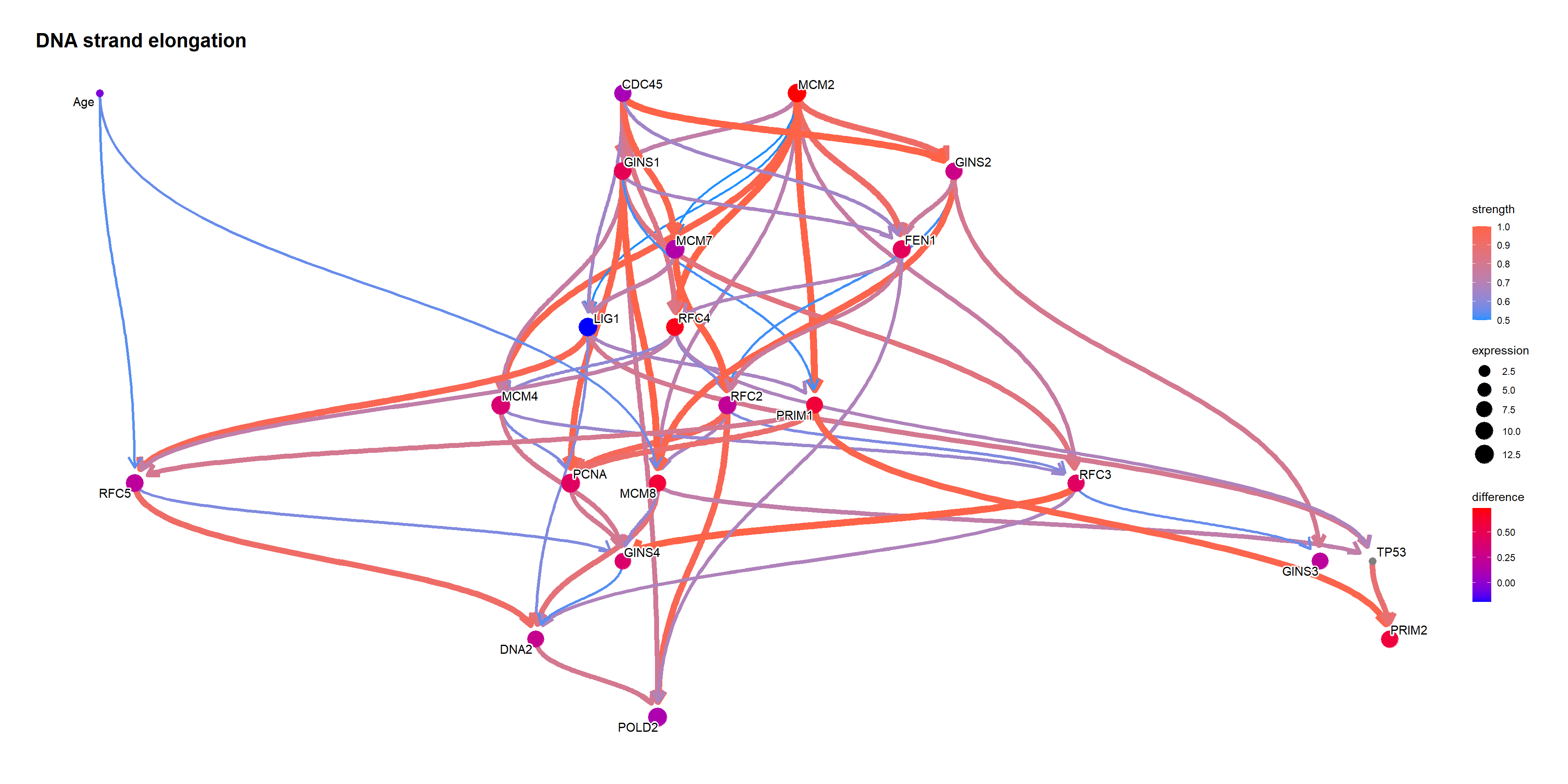

Perform likelihood weighting.

tp53low <- cpdist(topFit, nodes=candNodes, evidence=list(TP53 = 0), method="lw")
tp53high <- cpdist(topFit, nodes=candNodes, evidence=list(TP53 = 1), method="lw")

difMeanTp53 <- apply(tp53high, 2, function(x) weighted.mean(x, attributes(tp53high)$weights)) - apply(tp53low, 2, function(x) weighted.mean(x, attributes(tp53low)$weights))

changeCol <- topNet$plot$data
difMeanTp53 <- difMeanTp53[changeCol$name]

kable(head(difMeanTp53[order(abs(difMeanTp53), decreasing=T)]), col.names=c("difference"))

	difference
MCM2	0.5113805
RFC4	0.4569469
MCM8	0.4353333
PRIM1	0.4136929
PRIM2	0.3935092
GINS1	0.3680252

names(difMeanTp53) <- changeCol$name
changeCol$color <- difMeanTp53

## Replace shape and color
topNet$plot$data <- changeCol
topNet$plot + scale_color_continuous(low="blue",high="red",name="difference")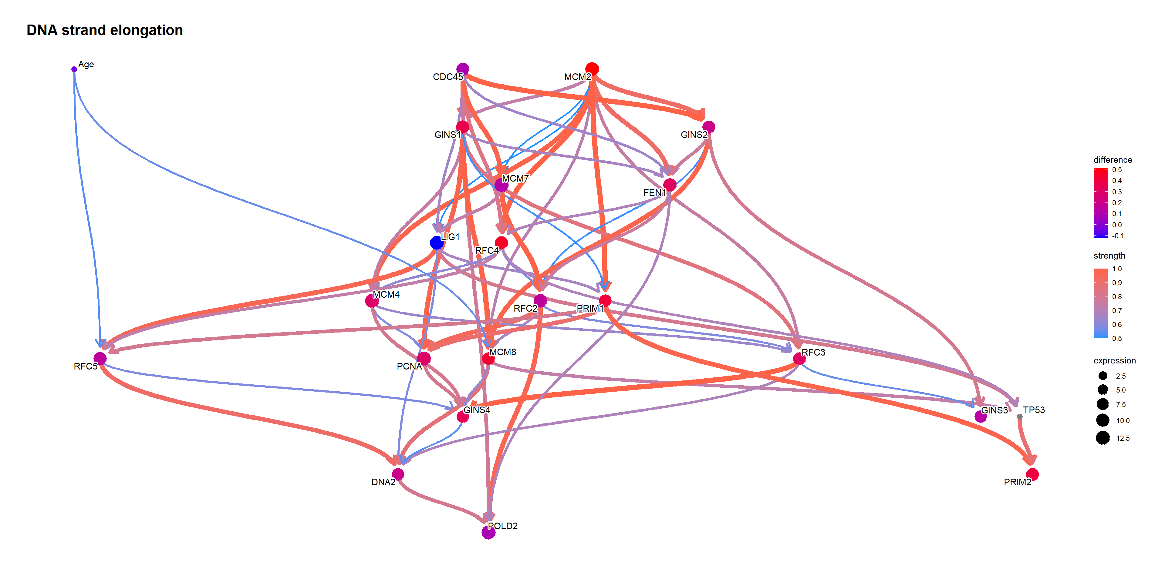

queryCpDistLw function performs sampling by likelihood weighting using cpdist, and returns the data.frame with weights. It just performs cpdist on the queried level and produce a plot. queryCpDistLs performs logic sampling.

## Only likelihood weighting is supported in queryCpDist.
q1 <- queryCpDistLw(topFit, names(difMeanTp53)[1], evidence="TP53", level=c(0,0.5,1))
kable(head(q1$df[,c(names(difMeanTp53)[1],"weights")]))

RFC2	weights
11.29786	0.8774882
10.16672	0.3570390
10.30900	0.2065809
10.82745	0.8837212
10.36271	0.8340634
10.50688	0.7633695

References

Cancer Genome Atlas Research Network, John N Weinstein, Eric A Collisson, Gordon B Mills, Kenna R Mills Shaw, Brad A Ozenberger, Kyle Ellrott, Ilya Shmulevich, Chris Sander, and Joshua M Stuart. 2013. “The Cancer Genome Atlas Pan-Cancer Analysis Project.” Nat. Genet. 45 (10): 1113–20.

Colaprico, Antonio, Tiago C Silva, Catharina Olsen, Luciano Garofano, Claudia Cava, Davide Garolini, Thais S Sabedot, et al. 2016. “TCGAbiolinks: An R/Bioconductor Package for Integrative Analysis of TCGA Data.” Nucleic Acids Res. 44 (8): e71.

Fouad, Hanan, Hosni Salem, Doha El-Sayed Ellakwa, and Manal Abdel-Hamid. 2019. “MMP-2 and MMP-9 as Prognostic Markers for the Early Detection of Urinary Bladder Cancer.” J. Biochem. Mol. Toxicol. 33 (4): e22275.

Han, A L, B A Veeneman, L El-Sawy, K C Day, M L Day, S A Tomlins, and E T Keller. 2017. “Fibulin-3 Promotes Muscle-Invasive Bladder Cancer.” Oncogene 36 (37): 5243–51.

Kuhn, Max. 2008. “Building Predictive Models in R Using the Caret Package.” Journal of Statistical Software, Articles 28 (5): 1–26.

Robin, Xavier, Natacha Turck, Alexandre Hainard, Natalia Tiberti, Frédérique Lisacek, Jean-Charles Sanchez, and Markus Müller. 2011. “pROC: An Open-Source Package for R and s+ to Analyze and Compare ROC Curves.” BMC Bioinformatics 12 (March): 77.

Vasala, Kaija, Paavo Pääkkö, and Taina Turpeenniemi-Hujanen. 2003. “Matrix Metalloproteinase-2 Immunoreactive Protein as a Prognostic Marker in Bladder Cancer.” Urology 62 (5): 952–57.

Winerdal, Malin E, David Krantz, Ciputra A Hartana, Ali A Zirakzadeh, Ludvig Linton, Emma A Bergman, Robert Rosenblatt, et al. 2018. “Urinary Bladder Cancer Tregs Suppress MMP2 and Potentially Regulate Invasiveness.” Cancer Immunol Res 6 (5): 528–38.